Module 1 — Regression on HPC#
DesignSafe AI Training

Sweeping M, L and E to learn the period equation#
Run one cantilever 75 times, changing three things each time — the tip mass \(M\), the column length \(L\), and the modulus \(E\) — and record the fundamental period \(T\) from the OpenSees eigen solve. Then fit a regression that predicts \(T\) from \((M, L, E)\).
The point is that we already know the answer, so the regression is checkable.
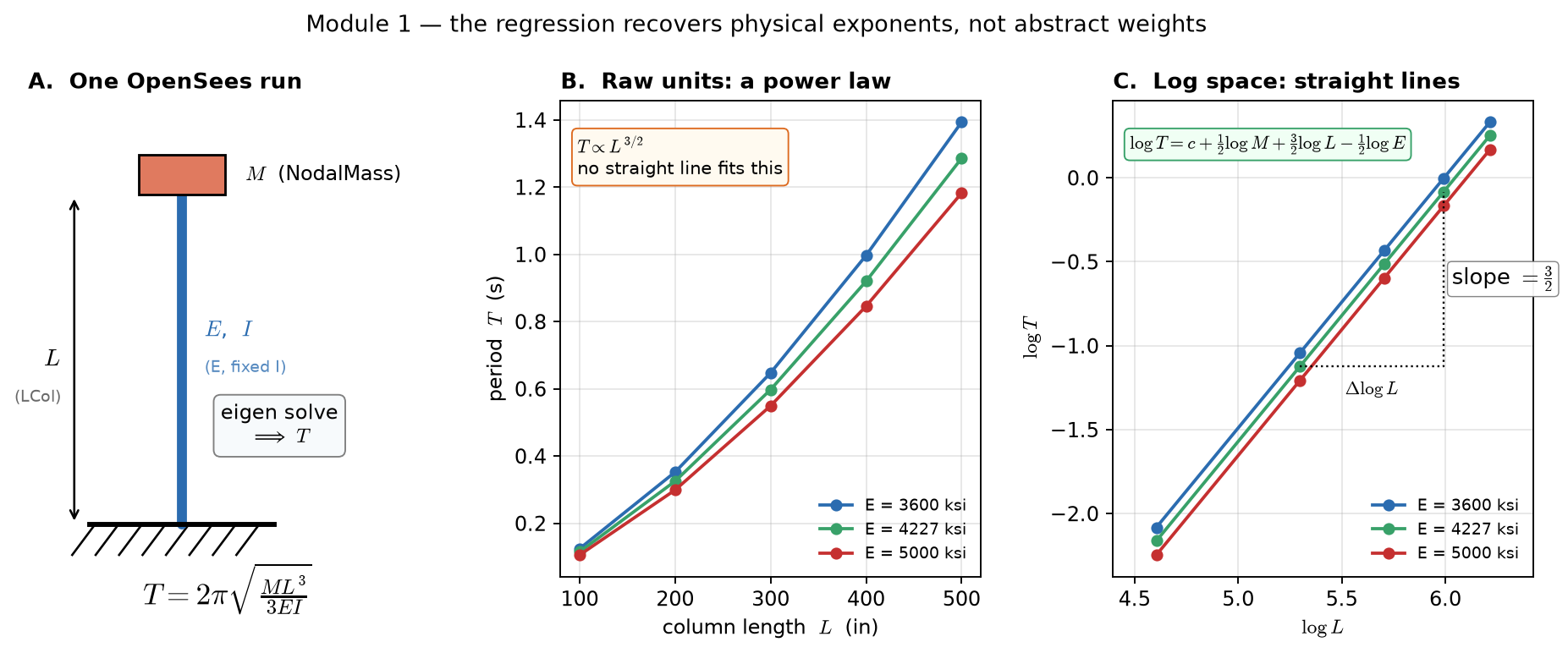
A cantilever’s period follows a power law#
A cantilever with a lumped tip mass has lateral stiffness \(k = 3EI/L^3\), so its period is
That is a power law — panel B above — and no straight line fits it.
Taking logarithms makes it linear#
\(T\) is a product of powers, so taking logarithms turns the products into sums and the exponents into slopes:
In log space the data falls on straight, parallel lines — panel C — which is exactly what ordinary least squares is built to fit.
So if we regress \(\log T\) on \(\log M\), \(\log L\), and \(\log E\), the three fitted coefficients should come out as \(+0.5\), \(+1.5\), and \(-0.5\). They are not abstract weights; they are the physical exponents of the period equation, and the model has to discover them from 75 simulations.
Exact physics turns the fit into a test of the whole workflow#
Because the physics is exact, the fit is a test of the whole workflow. Anything other than \([0.5,\ 1.5,\ -0.5]\) with \(R^2 = 1\) means the plumbing broke somewhere — the sweep, the staging, a task’s output, the aggregation. The recovered exponents check the pipeline end to end.
And the catch that sets up Module 2: this only worked because we knew to take the logarithms. Swap in a model with no closed form and no fixed feature basis is available.
75 runs, three log features, one log target#
Data |
75 OpenSeesPy pushover runs, one per grid point of |
Features |
\(\log M\), \(\log L\), \(\log E\) |
Target |
\(\log T\), the fundamental period from the OpenSees eigen solve |
Model |
Ordinary least squares (scikit-learn |
Split |
80/20 train/test (60/15 runs, fixed seed) |
Expected |
|
PyLauncher sweeps; a post-script fits the regression#
Sweep
NodalMass × LCol × Eover a 2D cantilever pushover in OpenSeesPy.Each combination runs as an independent PyLauncher task.
When all tasks finish,
ml_post.sh(the required post-script) aggregatesout_*/metrics.json, fits the regression on \(\log T\), and renders a diagnostic PDF/PNG.The archive holds the fitted model JSON, a per-task predictions CSV, a short report, and
opensees_ml_diagnostics.png.
The ML layer is a standard supervised pipeline: feature matrix → train/test split → linear fit → JSON model artifact → diagnostic figure. It trains on data the sweep generates, so it needs no external dataset.
This folder already contains the supporting files; the notebook does not rewrite them.
cantilever.py— one OpenSeesPy pushover taskaggregate_and_train.py— aggregation + regressionpostprocess.py— diagnostic plots (PDF/PNG)ml_post.sh— the required post-script; runs the aggregator and plotterrequirements.txt— extra packages for the job’s temp environmentsetup.sh— pre-script staging the TACC-compiled OpenSeesPy
Run this notebook from the folder that contains those files (e.g. copy the whole
folder into your ~/MyData/).
%pip install dapi --quiet
import os
from pathlib import Path
from dapi import DSClient

ds = DSClient()
input_dir = Path(os.getcwd())
print(f"Input directory: {input_dir}")
for fn in (
    "cantilever.py",
    "aggregate_and_train.py",
    "postprocess.py",
    "setup.sh",
    "ml_post.sh",
    "requirements.txt",
):
    assert (input_dir / fn).exists(), f"Missing: {fn}"
print("All required files present.")
/Users/krishna/.claude/jobs/791f8e64/tmp/mlrun/venv/lib/python3.14/site-packages/tqdm/auto.py:21: TqdmWarning: IProgress not found. Please update jupyter and ipywidgets. See https://ipywidgets.readthedocs.io/en/stable/user_install.html
  from .autonotebook import tqdm as notebook_tqdm
Authentication successful.
TMS credentials ready: frontera, stampede3, ls6
Input directory: /Users/krishna/.claude/jobs/791f8e64/tmp/mlrun/opensees_ml
All required files present.
Define the parameter sweep#
The three parameter lists combine into 5 × 5 × 3 = 75 tasks. Increase the lists for a bigger training set.
sweep = {
    "NODAL_MASS": [4.19, 4.39, 4.59, 4.79, 4.99],  # kip*s^2/in
    "LCOL": [100, 200, 300, 400, 500],  # in
    "EMOD": [
        3600,
        4227,
        5000,
    ],  # ksi
}

command = (
    "python3 cantilever.py --NodalMass NODAL_MASS --LCol LCOL --E EMOD "
    "--outDir out_NODAL_MASS_LCOL_EMOD"
)
Preview the sweep grid#
preview = ds.jobs.parametric_sweep.generate(command, sweep, preview=True)
print(f"Total runs: {len(preview)}")
preview.head()
Total runs: 75
| NODAL_MASS | LCOL | EMOD | |
|---|---|---|---|
| 0 | 4.19 | 100 | 3600 |
| 1 | 4.19 | 100 | 4227 |
| 2 | 4.19 | 100 | 5000 |
| 3 | 4.19 | 200 | 3600 |
| 4 | 4.19 | 200 | 4227 |
Write runsList.txt and call_pylauncher.py#
commands = ds.jobs.parametric_sweep.generate(command, sweep, str(input_dir))
print(f"Generated {len(commands)} task commands\n")
print("=== runsList.txt (first 5 lines) ===")
print("\n".join((input_dir / "runsList.txt").read_text().splitlines()[:5]))
print("...")
Generated 75 task commands

=== runsList.txt (first 5 lines) ===
python3 cantilever.py --NodalMass 4.19 --LCol 100 --E 3600 --outDir out_4.19_100_3600
python3 cantilever.py --NodalMass 4.19 --LCol 100 --E 4227 --outDir out_4.19_100_4227
python3 cantilever.py --NodalMass 4.19 --LCol 100 --E 5000 --outDir out_4.19_100_5000
python3 cantilever.py --NodalMass 4.19 --LCol 200 --E 3600 --outDir out_4.19_200_3600
python3 cantilever.py --NodalMass 4.19 --LCol 200 --E 4227 --outDir out_4.19_200_4227
...
Bundle the inputs into one ZIP#
Tapis stages each file of a directory input as its own transfer task (~40 s per file when the tenant transfer queue is busy), so eight loose files can spend minutes staging. Bundling them into a single inputs.zip, submitted from a directory containing only the bundle, turns eight transfers into one. The app expands it before anything else runs (UNZIP_INPUTS), so the pre-script, requirements file, and task scripts can all live inside the bundle.
import zipfile

staged_dir = input_dir / "staged"
staged_dir.mkdir(exist_ok=True)
bundle = staged_dir / "inputs.zip"

payload = [
    "cantilever.py",
    "aggregate_and_train.py",
    "postprocess.py",
    "setup.sh",
    "ml_post.sh",
    "requirements.txt",
    "runsList.txt",
    "call_pylauncher.py",
]
with zipfile.ZipFile(bundle, "w", zipfile.ZIP_DEFLATED) as zf:
    for fn in payload:
        zf.write(input_dir / fn, arcname=fn)
print(f"Bundled {len(payload)} files into {bundle} ({bundle.stat().st_size:,} bytes)")
Bundled 8 files into /Users/krishna/.claude/jobs/791f8e64/tmp/mlrun/opensees_ml/staged/inputs.zip (6,799 bytes)
Submit the job#
Set your TACC allocation, then run.
allocation = "DS-Portal-SPARC2026"  # <-- replace with your allocation

job = ds.jobs.parametric_sweep.submit(
    str(staged_dir),  # contains only inputs.zip — one staged transfer
    app_id="python-s3",
    allocation=allocation,
    node_count=1,
    cores_per_node=48,
    max_minutes=30,
    queue="skx-dev",
    extra_env_vars=[
        {"key": "UNZIP_INPUTS", "value": "inputs"},
        {"key": "EXTRA_MODULES", "value": "opensees,hdf5/1.14.4"},
        {"key": "PRE_SCRIPT", "value": "setup.sh"},
        {"key": "PIP_REQUIREMENTS", "value": "requirements.txt"},
        {"key": "POST_SCRIPT", "value": "ml_post.sh"},
        {"key": "POST_SCRIPT_REQUIRED", "value": "True"},
    ],
)
print(f"Job UUID: {job.uuid}")
job.monitor(interval=30, timeout_minutes=90)
Read the fitted model out of the job archive#
The fit should return the exponents of the period equation:
and \(R^2 = 1\) on the held-out runs, because the physics is exact and the only question is whether the pipeline delivered the data intact.
import json

archive_uri = job.archive_uri
print(f"Archive: {archive_uri}")
for item in ds.files.list(f"{archive_uri}/inputDirectory/ml_results"):
    print(f"  {item.name}")

job.download_output(
    "inputDirectory/ml_results/opensees_ml_model.json",
    "opensees_ml_model.json",
)
with open("opensees_ml_model.json") as f:
    model = json.load(f)
print(json.dumps(model, indent=2))
Archive: tapis://designsafe.storage.default/kks32/tapis-jobs-archive/2026-08-09Z/f370f8ba-d5dd-4e29-8e9d-ab492cc623da-007
  opensees_ml_diagnostics.pdf
  opensees_ml_diagnostics.png
  opensees_ml_model.json
  opensees_ml_preds.csv
  opensees_ml_report.txt
{
  "type": "linear_regression",
  "fitter": "sklearn",
  "target": "period",
  "target_space": "log",
  "feature_names": [
    "bias",
    "log_NodalMass",
    "log_LCol",
    "log_E"
  ],
  "coef": [
    -5.657664877475027,
    0.500000000000017,
    1.5000000000000022,
    -0.49999999999999106
  ],
  "r2_train": 1.0,
  "r2_test": 1.0,
  "n_train": 60,
  "n_test": 15,
  "seed": 12345
}
The fit recovers the coefficients#
From the verified Stampede3 run above (75 tasks, one SKX node, 42 s):
Coefficient |
Recovered |
Exact |
Meaning |
|---|---|---|---|
|
−5.657665 |
\(\log\!\left(2\pi/\sqrt{3I}\right)\) |
absorbs \(2\pi\) and the fixed \(I\) |
|
+0.500000 |
\(+\tfrac{1}{2}\) |
\(T \propto \sqrt{M}\) — heavier is slower |
|
+1.500000 |
\(+\tfrac{3}{2}\) |
\(T \propto L^{3/2}\) — the dominant term |
|
−0.500000 |
\(-\tfrac{1}{2}\) |
\(T \propto 1/\sqrt{E}\) — stiffer is faster |
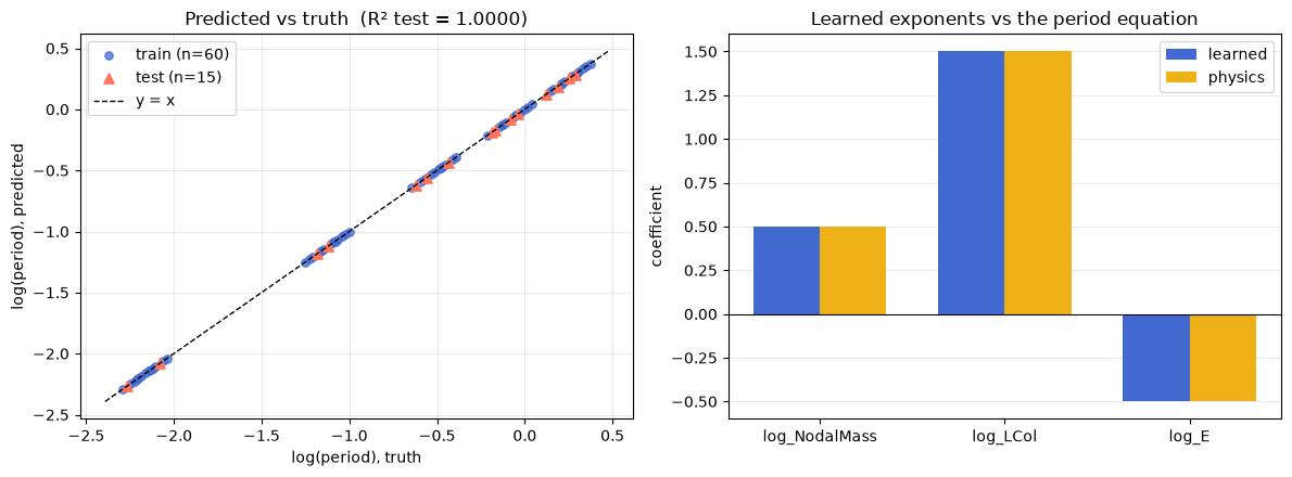
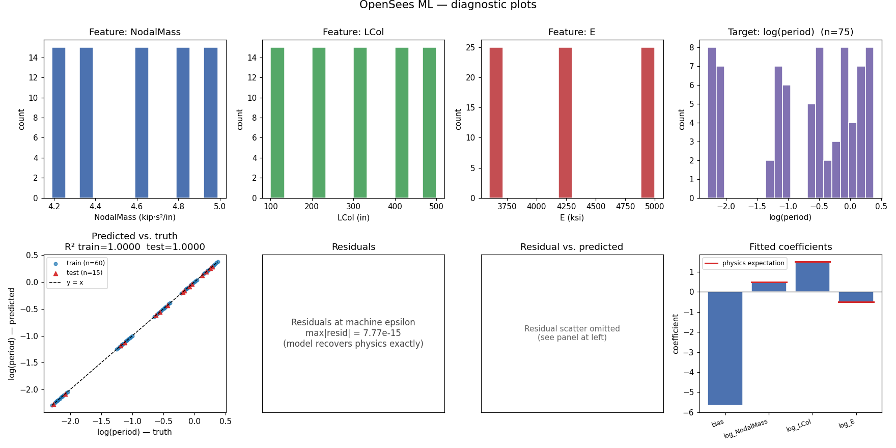
\(R^2 = 1.0000\) on both the 60 training and the 15 held-out test runs, with residuals at machine epsilon (\(\max|r| \approx 8 \times 10^{-15}\)).
The regression was never told the period equation. It saw
75 rows of (M, L, E, T) from independent OpenSees jobs and recovered
\(T = 2\pi\sqrt{ML^3/3EI}\) to fifteen significant figures — which simultaneously
confirms that the sweep, the staging, all 75 task outputs, and the aggregation are
correct. A single broken task would have shown up here.
Three coefficients, each one a physical exponent you can check by hand. Keep that standard in mind for Module 2, where the same data goes into a neural network and comes back as a few thousand weights that mean nothing on their own.
Diagnostic plots confirm residuals at machine epsilon#
postprocess.py runs on the compute node as part of ml_post.sh (the required post-script) and produces a 2×4 figure: feature histograms, target distribution, predicted-vs-truth scatter, residual panel, residual-vs-predicted, and a coefficient bar chart with the physics-expected exponents overlaid as red reference lines.
from IPython.display import Image, display

job.download_output(
    "inputDirectory/ml_results/opensees_ml_diagnostics.png",
    "opensees_ml_diagnostics.png",
)
display(Image("opensees_ml_diagnostics.png"))
Also download the PDF version (vector) and the per-task predictions CSV if you want to re-plot or do further analysis.
job.download_output(
    "inputDirectory/ml_results/opensees_ml_diagnostics.pdf",
    "opensees_ml_diagnostics.pdf",
)
job.download_output(
    "inputDirectory/ml_results/opensees_ml_preds.csv",
    "opensees_ml_preds.csv",
)
print("Downloaded diagnostics.pdf and preds.csv.")
Downloaded diagnostics.pdf and preds.csv.
Re-plot the predictions locally from the CSV#
ml_post.sh already rendered diagnostics on the compute node. The per-task predictions CSV supports custom analysis locally, so the cells below recreate two figures in the notebook. The first plots predicted versus truth colored by train/test split; the second sets the learned coefficients beside the physics expectation.
import matplotlib.pyplot as plt
import numpy as np
import pandas as pd

preds = pd.read_csv("opensees_ml_preds.csv")
train = preds[preds.split == "train"]
test = preds[preds.split == "test"]

fig, axes = plt.subplots(1, 2, figsize=(12, 4.5))

ax = axes[0]
ax.scatter(
    train.log_target,
    train.log_pred,
    s=28,
    color="#4269d0",
    alpha=0.75,
    label=f"train (n={len(train)})",
)
ax.scatter(
    test.log_target,
    test.log_pred,
    s=45,
    color="#ff725c",
    marker="^",
    label=f"test (n={len(test)})",
)
lims = [preds.log_target.min() - 0.1, preds.log_target.max() + 0.1]
ax.plot(lims, lims, "k--", lw=1, label="y = x")
ax.set_xlabel("log(period), truth")
ax.set_ylabel("log(period), predicted")
ax.set_title(f"Predicted vs truth  (R² test = {model['r2_test']:.4f})")
ax.legend()
ax.grid(alpha=0.25)
ax.set_axisbelow(True)

ax = axes[1]
names = model["feature_names"][1:]
learned = model["coef"][1:]
expected = [0.5, 1.5, -0.5]
x = np.arange(len(names))
ax.bar(x - 0.18, learned, 0.36, color="#4269d0", label="learned")
ax.bar(x + 0.18, expected, 0.36, color="#efb118", label="physics")
ax.set_xticks(x)
ax.set_xticklabels(names)
ax.axhline(0, color="k", lw=0.8)
ax.set_ylabel("coefficient")
ax.set_title("Learned exponents vs the period equation")
ax.legend()
ax.grid(alpha=0.25, axis="y")
ax.set_axisbelow(True)

fig.tight_layout()
plt.show()