
Module 4 — Physics-Informed Neural Networks#
DesignSafe AI Training


Fitting sparse data alone gets the boundary wrong#
Module 2 ended with a network fitted to eight deflection readings. It passed through all eight and was still wrong: the slope at the clamped support came out nonzero, and past the tip it wandered off. Adding two boundary terms to the loss fixed the support.
We also know the governing equation for that beam, and we ignored it.
This module puts the whole equation in the loss.
The network stops being a surrogate and becomes the solution#
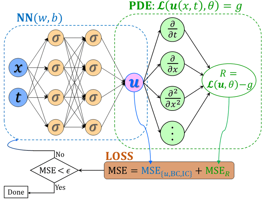
Everything in Modules 2 and 3 was a surrogate: fit a flexible function to input-output pairs, then interrogate it. A PINN is a different object.
Surrogate (Modules 2-3) |
PINN (this module) |
|
|---|---|---|
Network input |
design parameters \((M, L, E)\) |
a coordinate \(x\) |
Network output |
a quantity of interest |
the field \(w(x)\) |
Trained on |
labelled simulation runs |
the PDE residual |
Labelled data needed |
thousands |
zero (optional) |
The network is |
an approximation of a solver |
the solution itself |
That last row is the one to sit with. \(w_\theta(x)\) is not a model of the answer — it is a mesh-free ansatz for the answer, and training is the act of solving the differential equation.
| 5 | When PINNs are the wrong tool |
Setup#
%pip install torch matplotlib numpy --quiet
/private/tmp/claude-501/-Users-krishna-dev-DesignSafe-Training/a3c591bf-7af0-4642-a72e-3ed72e972147/scratchpad/venv/bin/python: No module named pip
Note: you may need to restart the kernel to use updated packages.
%matplotlib inline

import time

import numpy as np
import matplotlib.pyplot as plt
import torch
import torch.nn as nn

RNG = 42
torch.manual_seed(RNG)
np.random.seed(RNG)
torch.set_default_dtype(torch.float64)   # 2nd derivatives deserve float64

plt.rcParams.update({"figure.figsize": (11, 4), "font.size": 11})
print("torch", torch.__version__)
torch 2.13.0
A tip-loaded cantilever, in moment-curvature form#
Same cantilever as Module 2: tip-loaded, clamped at \(x = 0\).
We use the moment-curvature (second-order) form rather than \(EI\,w'''' = q\). Both describe the same beam, but the second-order form needs only two derivatives of the network instead of four — and every extra differentiation amplifies noise in the network’s output. We come back to the fourth-order version in Part 5.
The exact solution, for scoring ourselves:
First, non-dimensionalise — this is not optional#
With SI numbers, \(EI = 2\times10^{6}\) and the deflection is about \(0.02\). The residual \(EI\,w'' + P(L-x)\) has magnitude \(\sim\!5000\) while the quantity we want is \(\sim\!0.02\) — five orders of magnitude apart. Gradient descent on that is hopeless, and this is the single most common reason a hand-rolled PINN refuses to train.
Scale the problem instead. With
the equation becomes clean and \(O(1)\):
Everything below solves that. We convert back to millimetres only for plotting.
P, L, E, I = 1000.0, 5.0, 200e9, 1e-5      # N, m, Pa, m^4
EI = E * I
W_SCALE = P * L**3 / (3 * EI)               # tip deflection magnitude, m

print(f"EI       = {EI:.3e} N m^2")
print(f"W_SCALE  = {W_SCALE * 1000:.4f} mm   (tip deflection)")


def W_exact(xi):
    """Non-dimensional exact solution."""
    return -0.5 * (3 * xi**2 - xi**3)


def Wpp_exact(xi):
    """Its second derivative, = -3(1 - xi)."""
    return -3.0 * (1.0 - xi)


xi_plot = np.linspace(0, 1, 300)
print(f"\ncheck W_exact(1) = {W_exact(1.0):.4f}   (should be -1 by construction)")
print(f"physical tip     = {W_exact(1.0) * W_SCALE * 1000:.4f} mm")
EI       = 2.000e+06 N m^2
W_SCALE  = 20.8333 mm   (tip deflection)

check W_exact(1) = -1.0000   (should be -1 by construction)
physical tip     = -20.8333 mm
Part 1 — The residual, via automatic differentiation#
In Module 2 we differentiated a network with respect to its input to get \(\partial T/\partial L\). The same call, applied twice, gives us \(W''\).
The one detail that matters: create_graph=True. Without it the first derivative
is a leaf with no history, and the second grad call fails. With it, the
derivative is itself part of the graph — which is also what lets us
backpropagate through the residual to the weights.
def deriv(y, x, n=1):
    """n-th derivative of y with respect to x, keeping the graph alive."""
    for _ in range(n):
        y, = torch.autograd.grad(y, x, torch.ones_like(y), create_graph=True)
    return y


def make_net(width=32, depth=4):
    """tanh MLP. tanh because we need smooth 2nd derivatives -- ReLU's are 0."""
    layers, d = [], 1
    for _ in range(depth - 1):
        layers += [nn.Linear(d, width), nn.Tanh()]
        d = width
    layers += [nn.Linear(d, 1)]
    return nn.Sequential(*layers)


# Sanity check the machinery on a function whose derivatives we know.
xt = torch.linspace(0, 1, 5, requires_grad=True).unsqueeze(1)
y = -0.5 * (3 * xt**2 - xt**3)                      # W_exact, in torch
print("checking deriv() against the analytic W'' = -3(1 - xi):")
print("     xi       W2 (AD)   W2 (exact)")
for i, (a, b) in enumerate(zip(deriv(y, xt, 2).detach().numpy().ravel(),
                               Wpp_exact(xt.detach().numpy().ravel()))):
    print(f"  {xt[i].item():>5.2f} {a:>12.6f} {b:>12.6f}")
checking deriv() against the analytic W'' = -3(1 - xi):
     xi       W2 (AD)   W2 (exact)
   0.00    -3.000000    -3.000000
   0.25    -2.250000    -2.250000
   0.50    -1.500000    -1.500000
   0.75    -0.750000    -0.750000
   1.00     0.000000    -0.000000
Exact to machine precision — AD is not finite differences, there is no step size and no truncation error.
The residual needs no measured value of W#
The residual of \(W'' + 3(1-\xi) = 0\), evaluated at collocation points scattered through the domain. Note what is absent: any measured value of \(W\).
def pde_residual(model, xi):
    """r(xi) = W'' + 3(1 - xi). Zero when the beam equation is satisfied."""
    xi = xi.requires_grad_(True)
    W = model(xi)
    return deriv(W, xi, 2) + 3.0 * (1.0 - xi)


def physics_loss(model, xi_colloc):
    return (pde_residual(model, xi_colloc) ** 2).mean()
Part 2 — Solving the beam with no data#
The full loss has two parts and no data term at all:
This is the “soft” or penalty approach: the boundary conditions are encouraged, not enforced. \(\lambda_{BC}\) decides how much they matter relative to the equation, and choosing it is a genuine nuisance — we quantify that shortly.
def bc_loss(model):
    """Clamped end: W(0) = 0 and W'(0) = 0."""
    x0 = torch.zeros(1, 1, requires_grad=True)
    W0 = model(x0)
    dW0 = deriv(W0, x0, 1)
    return W0.squeeze() ** 2 + dW0.squeeze() ** 2


def train_soft(model, n_colloc=100, epochs=5000, lr=5e-3, lam_bc=100.0,
               resample=False, quiet=False):
    opt = torch.optim.Adam(model.parameters(), lr=lr)
    sched = torch.optim.lr_scheduler.CosineAnnealingLR(opt, T_max=epochs)
    xi_c = torch.linspace(0, 1, n_colloc).unsqueeze(1)
    hist = {"total": [], "pde": [], "bc": []}
    for ep in range(epochs):
        if resample:                       # fresh random collocation points
            xi_c = torch.rand(n_colloc, 1)
        opt.zero_grad()
        lp = physics_loss(model, xi_c.clone())
        lb = bc_loss(model)
        loss = lp + lam_bc * lb
        loss.backward()
        opt.step()
        sched.step()
        hist["total"].append(loss.item())
        hist["pde"].append(lp.item())
        hist["bc"].append(lb.item())
        if not quiet and ep % (epochs // 5) == 0:
            print(f"  epoch {ep:>5d}   pde {lp.item():.3e}   bc {lb.item():.3e}")
    return hist


torch.manual_seed(RNG)
soft = make_net()
t0 = time.time()
h_soft = train_soft(soft, lam_bc=100.0, epochs=5000)
t_soft = time.time() - t0
print(f"\ntrained in {t_soft:.1f} s using zero labelled data points")
epoch 0 pde 2.932e+00 bc 2.821e-03
epoch 1000 pde 9.193e-04 bc 3.409e-06
epoch 2000 pde 2.191e-04 bc 1.649e-11
epoch 3000 pde 8.922e-05 bc 7.990e-13
epoch 4000 pde 6.124e-05 bc 3.811e-13
trained in 4.6 s using zero labelled data points
def predict(model, xi_np):
    with torch.no_grad():
        return model(torch.tensor(xi_np).unsqueeze(1)).numpy().ravel()


W_soft = predict(soft, xi_plot)
err_soft = np.abs(W_soft - W_exact(xi_plot))

fig, ax = plt.subplots(1, 3, figsize=(14.5, 4))

ax[0].plot(xi_plot, W_exact(xi_plot) * W_SCALE * 1000, "k--", lw=2.5, label="exact")
ax[0].plot(xi_plot, W_soft * W_SCALE * 1000, "crimson", lw=2, label="PINN (no data)")
ax[0].set(xlabel=r"$\xi = x/L$", ylabel="deflection (mm)",
          title="Solved from the equation alone")
ax[0].legend(); ax[0].grid(alpha=.3)

ax[1].semilogy(h_soft["pde"], label="PDE residual")
ax[1].semilogy(h_soft["bc"], label="BC")
ax[1].set(xlabel="epoch", ylabel="loss", title="Loss components")
ax[1].legend(); ax[1].grid(alpha=.3)

ax[2].semilogy(xi_plot, np.maximum(err_soft, 1e-16))
ax[2].set(xlabel=r"$\xi$", ylabel=r"$|W_{PINN} - W_{exact}|$",
          title="Pointwise error")
ax[2].grid(alpha=.3)
plt.tight_layout(); plt.show()

print(f"max |error|  = {err_soft.max():.3e}  (non-dimensional)")
print(f"             = {err_soft.max() * W_SCALE * 1000:.5f} mm")
print(f"W(0)         = {predict(soft, np.array([0.0]))[0]:+.3e}   (should be exactly 0)")
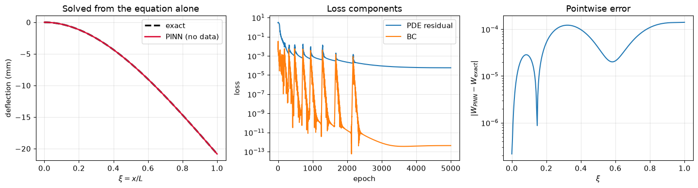
max |error|  = 1.411e-04  (non-dimensional)
             = 0.00294 mm
W(0)         = +2.150e-07   (should be exactly 0)
No labelled deflection anywhere in that loss. The network never saw a single value of \(W\) — only the requirement that its second derivative match \(-3(1-\xi)\), plus two conditions at the support. That is enough to pin the solution down.
Notice, though: \(W(0)\) is close to zero, not zero. The penalty pushed it down but nothing forced it. And we had to pick \(\lambda_{BC} = 100\) out of the air.
Raising \(\lambda_{BC}\) makes the solution worse, not better#
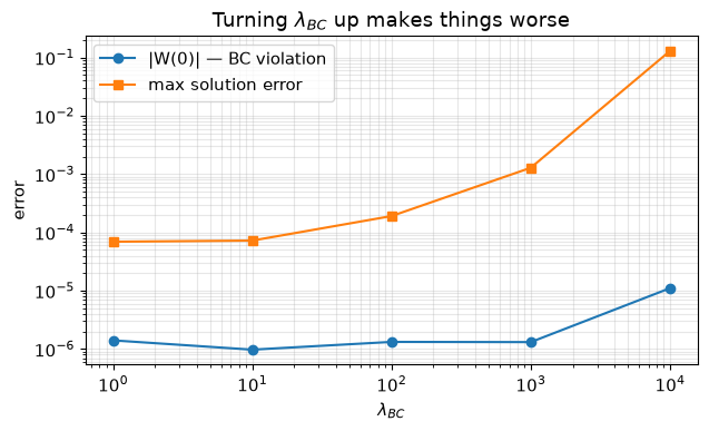
We picked 100 with no justification. Sweep it over four orders of magnitude and watch both error measures. (Shorter training here, 3000 epochs, so compare the columns against each other rather than against the run above.)
lams = [1.0, 10.0, 100.0, 1000.0, 10000.0]
rows = []
for lam in lams:
    torch.manual_seed(RNG)
    m = make_net()
    train_soft(m, lam_bc=lam, epochs=3000, quiet=True)
    Wp = predict(m, xi_plot)
    rows.append((lam, abs(predict(m, np.array([0.0]))[0]),
                 np.abs(Wp - W_exact(xi_plot)).max()))

print(f"  {'lambda_BC':>10s} {'|W(0)|':>12s} {'max |error|':>13s}")
for lam, bc, err in rows:
    print(f"  {lam:>10.0f} {bc:>12.2e} {err:>13.2e}")

fig, ax = plt.subplots(figsize=(6.5, 4))
ax.loglog(lams, [r[1] for r in rows], "o-", label="|W(0)| — BC violation")
ax.loglog(lams, [r[2] for r in rows], "s-", label="max solution error")
ax.set(xlabel=r"$\lambda_{BC}$", ylabel="error")
ax.set_title(r"Turning $\lambda_{BC}$ up makes things worse")
ax.legend(); ax.grid(True, which="both", alpha=.3)
plt.tight_layout(); plt.show()
   lambda_BC       |W(0)|   max |error|
           1     1.41e-06      6.92e-05
          10     9.75e-07      7.24e-05
         100     1.32e-06      1.91e-04
        1000     1.31e-06      1.28e-03
       10000     1.11e-05      1.29e-01
Read that table carefully, because it does not say what you might expect.
Raising \(\lambda_{BC}\) does not tighten the boundary condition. The BC violation sits at around \(10^{-6}\) for everything from \(\lambda = 1\) to \(\lambda = 1000\), and then gets worse at \(10^4\). Meanwhile the solution error climbs monotonically — by \(\lambda = 10^4\) it is roughly three orders of magnitude worse than at \(\lambda = 1\).
So on this problem the smallest weight wins on both counts, and the instinct many tutorials encourage — “use a big \(\lambda\) to really enforce the boundary conditions” — is actively destructive. Once \(\lambda\) dominates, the optimiser spends its steps on a term that was already satisfied and stops making progress on the equation.
Two honest conclusions:
\(\lambda_{BC}\) is a hyperparameter you have to sweep. Our original guess of 100 was already about 3x worse than \(\lambda = 1\), and nothing in the loss history would have told us.
Which way it should go is problem-dependent. Here the BC was easy to satisfy so a small weight sufficed. On a problem where the boundary fights the interior, the balance flips — and you would have to sweep again.
This is a well-known PINN failure mode: the loss terms have different scales and different curvature, so their gradients compete. The literature’s remedies are adaptive weighting (learn \(\lambda\) during training), gradient-norm balancing, and sequential training.
Or you can make the question disappear.
Part 3 — Hard constraints: make the BCs unbreakable#
Instead of penalising violations, build a network that cannot violate them.
Write the trial solution as
where \(N_\theta\) is an ordinary unconstrained MLP. Then, whatever the weights:
\(W_\theta(0) = 0^2 \cdot N(0) = 0\) — the deflection BC, exactly.
\(W_\theta'(\xi) = 2\xi N + \xi^2 N'\), so \(W_\theta'(0) = 0\) — the rotation BC, exactly.
The factor \(\xi^2\) is not arbitrary: a clamped end needs two conditions, and \(\xi^2\) has a double root there. A simple support (only \(W = 0\)) would take \(\xi^1\); a domain clamped at both ends would take \(\xi^2(1-\xi)^2\).
Both boundary conditions now hold identically, so they leave the loss entirely:
One term. No \(\lambda\) to tune.
class HardBC(nn.Module):
    """W(xi) = xi^2 * N(xi), so W(0) = W'(0) = 0 by construction."""

    def __init__(self, base):
        super().__init__()
        self.base = base

    def forward(self, xi):
        return xi**2 * self.base(xi)


def train_hard(model, n_colloc=100, epochs=5000, lr=5e-3, quiet=False):
    opt = torch.optim.Adam(model.parameters(), lr=lr)
    sched = torch.optim.lr_scheduler.CosineAnnealingLR(opt, T_max=epochs)
    xi_c = torch.linspace(0, 1, n_colloc).unsqueeze(1)
    hist = {"pde": []}
    for ep in range(epochs):
        opt.zero_grad()
        lp = physics_loss(model, xi_c.clone())
        lp.backward()
        opt.step()
        sched.step()
        hist["pde"].append(lp.item())
        if not quiet and ep % (epochs // 5) == 0:
            print(f"  epoch {ep:>5d}   pde {lp.item():.3e}")
    return hist


torch.manual_seed(RNG)
hard = HardBC(make_net())
t0 = time.time()
h_hard = train_hard(hard, epochs=5000)
t_hard = time.time() - t0
print(f"\ntrained in {t_hard:.1f} s")
epoch 0 pde 3.349e+00
epoch 1000 pde 4.813e-06
epoch 2000 pde 4.106e-06
epoch 3000 pde 3.673e-06
epoch 4000 pde 3.402e-06
trained in 4.0 s
W_hard = predict(hard, xi_plot)
err_hard = np.abs(W_hard - W_exact(xi_plot))

x0 = torch.zeros(1, 1, requires_grad=True)
W0_hard = hard(x0)
slope0 = deriv(W0_hard, x0, 1)

print("                       soft (lambda=100)        hard (xi^2 * N)")
print(f"  |W(0)|          {abs(predict(soft, np.array([0.0]))[0]):>18.3e} "
      f"{abs(float(W0_hard.detach())):>22.3e}")
print(f"  |W'(0)|         {'(not enforced)':>18s} {abs(float(slope0.detach())):>22.3e}")
print(f"  max |error|     {err_soft.max():>18.3e} {err_hard.max():>22.3e}")
print(f"  loss terms      {'2 (+ lambda)':>18s} {'1':>22s}")

fig, ax = plt.subplots(1, 2, figsize=(12.5, 4.2))
ax[0].plot(xi_plot, W_exact(xi_plot) * W_SCALE * 1000, "k--", lw=2.5, label="exact")
ax[0].plot(xi_plot, W_soft * W_SCALE * 1000, lw=1.8, alpha=.8, label="soft BC")
ax[0].plot(xi_plot, W_hard * W_SCALE * 1000, lw=1.8, label="hard BC")
ax[0].set(xlabel=r"$\xi$", ylabel="deflection (mm)", title="Both solve the beam")
ax[0].legend(); ax[0].grid(alpha=.3)

ax[1].semilogy(xi_plot, np.maximum(err_soft, 1e-18), label="soft BC")
ax[1].semilogy(xi_plot, np.maximum(err_hard, 1e-18), label="hard BC")
ax[1].set(xlabel=r"$\xi$", ylabel="absolute error", title="Error, note the support")
ax[1].legend(); ax[1].grid(alpha=.3)
plt.tight_layout(); plt.show()
                       soft (lambda=100)        hard (xi^2 * N)
  |W(0)|                   2.150e-07              0.000e+00
  |W'(0)|             (not enforced)              0.000e+00
  max |error|              1.411e-04              3.626e-05
  loss terms            2 (+ lambda)                      1
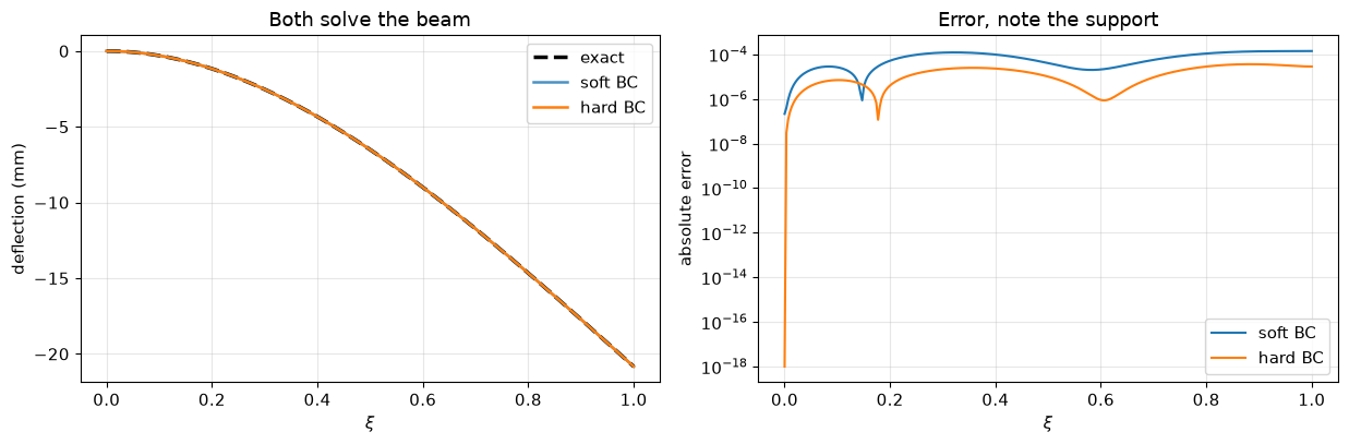
The hard-constrained network satisfies both boundary conditions to machine precision — because they are algebraic identities, not optimisation targets — and it has one fewer hyperparameter.
Use hard constraints whenever the geometry lets you. It is the highest value-per-line change in this notebook. The limitation is that you need a distance function you can write down, which is easy on intervals and boxes and awkward on complicated domains.
Part 4 — The inverse problem: what PINNs are actually for#
Parts 2 and 3 solved a problem a first-year student solves by integrating twice, and we will be honest about that in Part 5. Here is the case where the PINN earns its keep.
The real situation. You have a beam in the field. You can measure deflection at a handful of points. You do not know its stiffness — the section has corroded, or the concrete’s modulus is uncertain, or it is a soil profile rather than a beam. You want \(EI\).
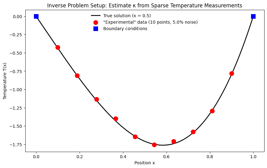
This is hard for a classical solver: it is an optimisation around a forward solve, one solve per iteration. For a PINN it is almost free — make the unknown a trainable parameter and let the same gradient descent that fits the network also fit the physics.
Write the scaled equation with the unknown exposed. With \(\tilde w = w/w_{ref}\) for a fixed reference scale \(w_{ref}\),
Recover \(\kappa\), and \(EI = PL^3 / (\kappa\, w_{ref})\) follows.
We optimise \(\log \kappa\) rather than \(\kappa\): it keeps \(\kappa\) positive automatically and makes the step size scale-free.
W_REF = 0.02                     # m, a round number near the measured scale
KAPPA_TRUE = P * L**3 / (EI * W_REF)
print(f"true kappa = {KAPPA_TRUE:.4f}   (this is the answer we must recover)")
print(f"true EI    = {EI:.4e} N m^2")
print(f"true E     = {E / 1e9:.1f} GPa")

# Eight noisy sensor readings, in the scaled variable.
N_SENS, NOISE_MM = 8, 0.15
rng = np.random.default_rng(RNG)
xi_s = np.linspace(0.15, 1.0, N_SENS)          # no sensor at the clamp
w_true_mm = W_exact(xi_s) * W_SCALE * 1000
w_meas_mm = w_true_mm + NOISE_MM * rng.standard_normal(N_SENS)

xi_sens = torch.tensor(xi_s).unsqueeze(1)
w_sens = torch.tensor(w_meas_mm / 1000.0 / W_REF).unsqueeze(1)

print(f"\n{N_SENS} readings with {NOISE_MM} mm noise "
      f"({NOISE_MM / abs(w_true_mm).max() * 100:.1f}% of tip deflection)")
for a, b in zip(w_true_mm, w_meas_mm):
    print(f"    true {a:>8.3f} mm    measured {b:>8.3f} mm")
true kappa = 3.1250   (this is the answer we must recover)
true EI    = 2.0000e+06 N m^2
true E     = 200.0 GPa

8 readings with 0.15 mm noise (0.7% of tip deflection)
    true   -0.668 mm    measured   -0.622 mm
    true   -2.094 mm    measured   -2.250 mm
    true   -4.191 mm    measured   -4.079 mm
    true   -6.848 mm    measured   -6.707 mm
    true   -9.953 mm    measured  -10.246 mm
    true  -13.393 mm    measured  -13.589 mm
    true  -17.057 mm    measured  -17.038 mm
    true  -20.833 mm    measured  -20.881 mm
class InversePINN(nn.Module):
    """Hard-BC network plus a trainable log(kappa)."""

    def __init__(self, base, kappa_init=1.0):
        super().__init__()
        self.base = base
        self.log_kappa = nn.Parameter(torch.tensor(float(np.log(kappa_init))))

    @property
    def kappa(self):
        return torch.exp(self.log_kappa)

    def forward(self, xi):
        return xi**2 * self.base(xi)          # w(0) = w'(0) = 0, exactly


def inverse_residual(model, xi):
    xi = xi.requires_grad_(True)
    w = model(xi)
    return deriv(w, xi, 2) + model.kappa * (1.0 - xi)


def train_inverse(model, xi_sens, w_sens, epochs=8000, lr=5e-3,
                  n_colloc=100, lam_data=100.0, quiet=False):
    opt = torch.optim.Adam(model.parameters(), lr=lr)
    sched = torch.optim.lr_scheduler.CosineAnnealingLR(opt, T_max=epochs)
    xi_c = torch.linspace(0, 1, n_colloc).unsqueeze(1)
    hist = {"data": [], "pde": [], "kappa": []}
    for ep in range(epochs):
        opt.zero_grad()
        l_pde = (inverse_residual(model, xi_c.clone()) ** 2).mean()
        l_dat = ((model(xi_sens) - w_sens) ** 2).mean()
        (l_pde + lam_data * l_dat).backward()
        opt.step()
        sched.step()
        hist["pde"].append(l_pde.item())
        hist["data"].append(l_dat.item())
        hist["kappa"].append(float(model.kappa.detach()))
        if not quiet and ep % (epochs // 5) == 0:
            print(f"  epoch {ep:>5d}   data {l_dat.item():.2e}   "
                  f"pde {l_pde.item():.2e}   kappa {hist['kappa'][-1]:.4f}")
    return hist


torch.manual_seed(RNG)
inv = InversePINN(make_net(), kappa_init=1.0)     # start deliberately wrong
print(f"starting kappa = {float(inv.kappa.detach()):.4f}  (true {KAPPA_TRUE:.4f})\n")
h_inv = train_inverse(inv, xi_sens, w_sens, epochs=8000)
starting kappa = 1.0000  (true 3.1250)

  epoch     0   data 3.73e-01   pde 4.53e-01   kappa 0.9950
epoch 1600 data 4.99e-05 pde 5.92e-05 kappa 3.1382
epoch 3200 data 4.98e-05 pde 4.90e-05 kappa 3.1383
epoch 4800 data 4.98e-05 pde 4.33e-05 kappa 3.1384
epoch 6400 data 4.97e-05 pde 4.38e-05 kappa 3.1384
kappa_hat = float(inv.kappa.detach())
EI_hat = P * L**3 / (kappa_hat * W_REF)
E_hat = EI_hat / I

print(f"  {'':<12s} {'recovered':>14s} {'true':>14s} {'error':>9s}")
print(f"  {'kappa':<12s} {kappa_hat:>14.4f} {KAPPA_TRUE:>14.4f} "
      f"{abs(kappa_hat/KAPPA_TRUE - 1)*100:>8.2f}%")
print(f"  {'EI (N m^2)':<12s} {EI_hat:>14.4e} {EI:>14.4e} "
      f"{abs(EI_hat/EI - 1)*100:>8.2f}%")
print(f"  {'E (GPa)':<12s} {E_hat/1e9:>14.2f} {E/1e9:>14.2f} "
      f"{abs(E_hat/E - 1)*100:>8.2f}%")

fig, ax = plt.subplots(1, 3, figsize=(15, 4))

ax[0].axhline(KAPPA_TRUE, color="k", ls="--", lw=2, label=r"true $\kappa$")
ax[0].plot(h_inv["kappa"], color="crimson", lw=1.8, label=r"$\kappa$ during training")
ax[0].set(xlabel="epoch", ylabel=r"$\kappa$",
          title="The unknown converges alongside the weights")
ax[0].legend(); ax[0].grid(alpha=.3)

w_inv = predict(inv, xi_plot) * W_REF * 1000
ax[1].plot(xi_plot, W_exact(xi_plot) * W_SCALE * 1000, "k--", lw=2.5, label="true beam")
ax[1].plot(xi_plot, w_inv, color="teal", lw=2, label="inverse PINN")
ax[1].scatter(xi_s, w_meas_mm, s=70, color="gold", edgecolor="k",
              zorder=5, label=f"{N_SENS} noisy readings")
ax[1].set(xlabel=r"$\xi$", ylabel="deflection (mm)",
          title="Field recovered, stiffness identified")
ax[1].legend(fontsize=9); ax[1].grid(alpha=.3)

ax[2].semilogy(h_inv["data"], label="data misfit")
ax[2].semilogy(h_inv["pde"], label="PDE residual")
ax[2].set(xlabel="epoch", ylabel="loss", title="Loss components")
ax[2].legend(); ax[2].grid(alpha=.3)
plt.tight_layout(); plt.show()
                    recovered           true     error
  kappa                3.1384         3.1250     0.43%
  EI (N m^2)       1.9914e+06     2.0000e+06     0.43%
  E (GPa)              199.14         200.00     0.43%
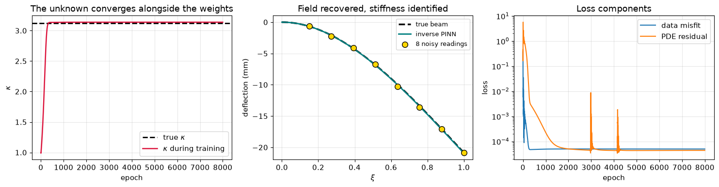
Eight noisy readings, no knowledge of the stiffness, and we recovered \(EI\) — and got the full deflection field as a by-product, including at the support where we never measured.
This is the honest headline for PINNs. Compare the alternatives:
Classical inverse solve |
PINN |
|
|---|---|---|
Structure |
outer optimiser wrapping a forward solver |
one gradient descent |
Cost |
one full solve per iteration |
one backward pass per iteration |
Sparse, noisy data |
needs regularisation bolted on |
the PDE is the regulariser |
Extra unknown fields |
often intractable |
another |
The last row is the real prize: if the stiffness varied along the span, \(EI(x)\), you would replace the scalar parameter with a second small network and change almost nothing else.
optional — how much does the noise cost you?#
Repeat the identification at several noise levels to see how the estimate degrades. This is the number a reviewer will ask for.
noise_levels = [0.0, 0.05, 0.15, 0.4]
out = []
for nz in noise_levels:
    r = np.random.default_rng(RNG)
    meas = W_exact(xi_s) * W_SCALE * 1000 + nz * r.standard_normal(N_SENS)
    ws = torch.tensor(meas / 1000.0 / W_REF).unsqueeze(1)
    torch.manual_seed(RNG)
    m = InversePINN(make_net(), kappa_init=1.0)
    train_inverse(m, xi_sens, ws, epochs=5000, quiet=True)
    k = float(m.kappa.detach())
    out.append((nz, k, P * L**3 / (k * W_REF) / I / 1e9))

print(f"  {'noise (mm)':>11s} {'kappa':>9s} {'E (GPa)':>9s} {'E error':>9s}")
for nz, k, e in out:
    print(f"  {nz:>11.2f} {k:>9.4f} {e:>9.2f} {abs(e*1e9/E - 1)*100:>8.1f}%")
   noise (mm)     kappa   E (GPa)   E error
         0.00    3.1248    200.01      0.0%
         0.05    3.1293    199.73      0.1%
         0.15    3.1383    199.15      0.4%
         0.40    3.1609    197.73      1.1%
Part 5 — When PINNs are the wrong tool#
Training-course notebooks tend to stop at “it worked”. Three caveats that decide whether you should use this in real work.
1. As a forward solver, PINNs lose to FEM. Badly.#
Our forward problem has an exact two-element FEM answer. Let’s time it.
# Exact solution by direct integration -- what a solver actually does.
t0 = time.time()
w_direct = W_exact(xi_plot)
t_direct = time.time() - t0

print(f"  analytic / FEM   {t_direct * 1e6:>10.1f} us    error 0 (exact)")
print(f"  PINN (soft BC)   {t_soft:>10.2f} s     error {err_soft.max():.2e}")
print(f"  PINN (hard BC)   {t_hard:>10.2f} s     error {err_hard.max():.2e}")
print(f"\n  PINN is ~{t_hard / max(t_direct, 1e-9):,.0f}x slower and less accurate.")
  analytic / FEM         45.1 us    error 0 (exact)
  PINN (soft BC)         4.57 s     error 1.41e-04
  PINN (hard BC)         3.96 s     error 3.63e-05

  PINN is ~87,922x slower and less accurate.
That ratio is not a bug and it does not go away with tuning. A PINN solves a global optimisation problem where FEM solves a sparse linear system, and for a well-posed forward problem on a simple domain the linear system wins every time.
So do not sell a PINN as a faster solver. Reach for one when it offers something FEM does not:
Inverse problems and data assimilation — Part 4. Unknown coefficients, sparse noisy measurements, no clean boundary data.
Filling in missing physics — part of the model is known, part is learned.
High-dimensional parametric PDEs — where meshing is the bottleneck.
Awkward geometry or moving boundaries — no mesh to generate or remesh.
2. Higher derivatives get expensive and noisy#
We deliberately used \(EI\,w'' = M(x)\) rather than \(EI\,w'''' = q\). Each extra derivative means another backward pass through the graph and amplifies the network’s own wiggle. Here is the fourth derivative of our trained network, which should be exactly zero for a tip-loaded beam (\(q = 0\)).
xi_d = torch.linspace(0.02, 0.98, 200, requires_grad=True).unsqueeze(1)
Wd = hard(xi_d)
d2 = deriv(Wd, xi_d, 2).detach().numpy().ravel()
d4 = deriv(hard(xi_d), xi_d, 4).detach().numpy().ravel()
xg = xi_d.detach().numpy().ravel()

fig, ax = plt.subplots(1, 2, figsize=(12.5, 4))
ax[0].plot(xg, Wpp_exact(xg), "k--", lw=2.5, label="exact $W''$")
ax[0].plot(xg, d2, color="teal", lw=1.8, label="AD $W''$")
ax[0].set(xlabel=r"$\xi$", ylabel=r"$W''$", title="2nd derivative: clean")
ax[0].legend(); ax[0].grid(alpha=.3)

ax[1].axhline(0, color="k", ls="--", lw=2.5, label="exact $W'''' = 0$")
ax[1].plot(xg, d4, color="crimson", lw=1.2, label="AD $W''''$")
ax[1].set(xlabel=r"$\xi$", ylabel=r"$W''''$",
          title="4th derivative: noisy, and never trained")
ax[1].legend(); ax[1].grid(alpha=.3)
plt.tight_layout(); plt.show()

print(f"  max |W''  - exact| = {np.abs(d2 - Wpp_exact(xg)).max():.3e}")
print(f"  max |W''''|        = {np.abs(d4).max():.3e}   (should be 0)")
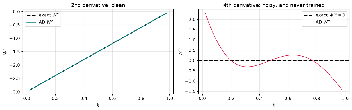
  max |W''  - exact| = 2.680e-03
  max |W''''|        = 2.306e+00   (should be 0)
The second derivative — the one in the loss — is accurate. The fourth, which nothing constrained, is orders of magnitude worse. A PINN is only accurate in the quantities you put in the loss. If you need bending moments, constrain moments; do not differentiate a displacement network twice more and hope.
For genuinely fourth-order problems the usual fix is a mixed formulation: two networks, one for \(w\) and one for \(M\), coupled by \(EI w'' = M\) and \(M'' = q\). Two second derivatives instead of one fourth.
3. Spectral bias#
Networks learn smooth, low-frequency structure first and high-frequency structure slowly or never. Our beam is a cubic, so this never bit us. A problem with sharp gradients — a shock, a boundary layer, a liquefaction front — will train far more reluctantly, and the standard tools are Fourier features, domain decomposition, and curriculum training on frequency.
One trained PINN serves exactly one load case#
Look back at what we produced: one deflection field, for one load case.
Change \(P\), and every weight is wrong. Change the load from a tip force to a distributed pressure and you retrain from scratch — minutes of optimisation for each new load, where a surrogate is supposed to evaluate instantly.
A design study sweeps hundreds of load cases. A PINN, as built here, cannot serve one.
That is what operator learning fixes.
Summary#
The network is the solution |
Input a coordinate, output a field. Training is solving the PDE. |
Non-dimensionalise first |
Raw SI put the residual \(10^5\) above the solution. This is the most common reason a PINN will not train. |
Zero labelled data is enough |
The residual plus boundary conditions pinned down the beam completely. |
Soft BCs bring a hyperparameter you cannot win |
No \(\lambda_{BC}\) minimised both BC violation and solution error. |
Hard constraints are strictly better where available |
\(W = \xi^2 N(\xi)\) satisfies the clamped end exactly and deletes \(\lambda\). |
Inverse problems are the real application |
\(EI\) from 8 noisy readings, as one extra |
Accurate only where constrained |
\(W''\) was excellent; the unconstrained \(W''''\) was garbage. |
Not a faster forward solver |
Orders of magnitude slower than FEM here, and less accurate. Be honest about this. |
Go deeper#
SciML — Burgers’ equation — a nonlinear, shock-forming case
DesignSafe PINN training — heat transfer and Burgers notebooks
Raissi, Perdikaris & Karniadakis (2019), Physics-informed neural networks — the original paper