
Operator learning, part A — the 1D Darcy problem#
DesignSafe AI Training

Ported from the SciML course (Krishna Kumar).
The PINN notebooks solved one problem for one right-hand side. Change it and every weight is wrong. Here we learn the solution operator instead — a map from one function to another, so any new input function is a forward pass.
# Capture figures as notebook outputs. The course notebooks run in a
# live JupyterLab where this is implicit; the published book renders
# saved outputs, so without it every plot is lost.
%matplotlib inline
import numpy as np
import warnings
import torch
import torch.nn as nn
import torch.optim as optim
from tqdm import tqdm
import matplotlib.pyplot as plt
from torch.utils.data import DataLoader, TensorDataset

warnings.filterwarnings('ignore')

# Set style and random seeds
np.random.seed(42)
torch.manual_seed(42)

# Device selection
def get_device():
    if torch.cuda.is_available():
        return torch.device("cuda")
    elif torch.backends.mps.is_available():
        return torch.device("mps")
    else:
        return torch.device("cpu")

device = get_device()
print(f"Using device: {device}")
Using device: mps
From Scalars to Functions - The Conceptual Leap#
Let’s start with something familiar and build our intuition.
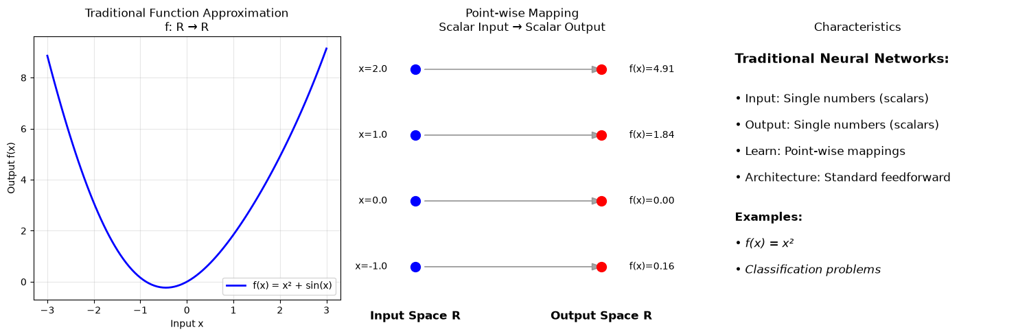
Traditional Function Approximation#
We know neural networks can learn mappings like:
Input: A number \(x = 2.5\)
Output: A number \(f(x) = x^2 = 6.25\)
This is point-wise mapping: each input point maps to an output point.
Operator Learning: The Next Level#
Now imagine:
Input: An entire function \(u(x) = \sin(x)\)
Output: Another entire function \(\mathcal{G}[u](x) = \cos(x)\) (the derivative!)
This is function-to-function mapping: each input function maps to an output function.
Examples of operators we encounter in science:
Derivative operator: \(\mathcal{D}[u] = \frac{du}{dx}\)
Integration operator: \(\mathcal{I}[f] = \int_0^x f(t) dt\)
PDE solution operator: Given source \(f\), return solution \(u\) of \(\nabla^2 u = f\)
def demonstrate_function_approximation():
    """Show traditional function approximation with clearer visualization"""

    # Example: Learn f(x) = x² + sin(x)
    x = np.linspace(-3, 3, 100)
    y = x**2 + np.sin(x)

    plt.figure(figsize=(15, 5))

    # Plot 1: Traditional function plot
    plt.subplot(1, 3, 1)
    plt.plot(x, y, 'b-', linewidth=2, label='f(x) = x² + sin(x)')
    plt.title('Traditional Function Approximation\nf: R → R')
    plt.xlabel('Input x')
    plt.ylabel('Output f(x)')
    plt.grid(True, alpha=0.3)
    plt.legend()

    # Plot 2: Point-wise mapping visualization (improved)
    plt.subplot(1, 3, 2)

    # Show specific input-output pairs
    sample_x = np.array([-1.0, 0.0, 1.0, 2.0])
    sample_y = sample_x**2 + np.sin(sample_x)

    # Create a clearer mapping visualization
    input_positions = np.arange(len(sample_x))
    output_positions = np.arange(len(sample_x)) + 0.5

    # Plot input values
    for i, (xi, yi) in enumerate(zip(sample_x, sample_y)):
        # Input side
        plt.scatter(0, input_positions[i], s=100, c='blue', zorder=5)
        plt.text(-0.3, input_positions[i], f'x={xi:.1f}', ha='right', va='center')

        # Output side
        plt.scatter(2, input_positions[i], s=100, c='red', zorder=5)
        plt.text(2.3, input_positions[i], f'f(x)={yi:.2f}', ha='left', va='center')

        # Arrow showing mapping
        plt.arrow(0.1, input_positions[i], 1.8, 0,
                 head_width=0.1, head_length=0.1, fc='gray', ec='gray', alpha=0.7)

    plt.xlim(-0.5, 2.8)
    plt.ylim(-0.5, len(sample_x) - 0.5)
    plt.title('Point-wise Mapping\nScalar Input → Scalar Output')
    plt.text(0, -0.8, 'Input Space R', ha='center', fontsize=12, fontweight='bold')
    plt.text(2, -0.8, 'Output Space R', ha='center', fontsize=12, fontweight='bold')
    plt.axis('off')

    # Plot 3: Characteristics
    plt.subplot(1, 3, 3)
    plt.text(0.1, 0.9, 'Traditional Neural Networks:', fontsize=14, fontweight='bold',
             transform=plt.gca().transAxes)
    plt.text(0.1, 0.75, '• Input: Single numbers (scalars)', fontsize=12,
             transform=plt.gca().transAxes)
    plt.text(0.1, 0.65, '• Output: Single numbers (scalars)', fontsize=12,
             transform=plt.gca().transAxes)
    plt.text(0.1, 0.55, '• Learn: Point-wise mappings', fontsize=12,
             transform=plt.gca().transAxes)
    plt.text(0.1, 0.45, '• Architecture: Standard feedforward', fontsize=12,
             transform=plt.gca().transAxes)
    plt.text(0.1, 0.3, 'Examples:', fontsize=12, fontweight='bold',
             transform=plt.gca().transAxes)
    plt.text(0.1, 0.2, '• f(x) = x²', fontsize=12,
             transform=plt.gca().transAxes, style='italic')
    plt.text(0.1, 0.1, '• Classification problems', fontsize=12,
             transform=plt.gca().transAxes, style='italic')
    plt.xlim(0, 1)
    plt.ylim(0, 1)
    plt.axis('off')
    plt.title('Characteristics')

    plt.tight_layout()
    plt.show()

    print("Traditional Function Approximation:")
    print("• Takes individual points as input")
    print("• Produces individual points as output")
    print("• Neural network learns: x → f(x)")
    print("• This is what we're familiar with!")

demonstrate_function_approximation()
Traditional Function Approximation:
• Takes individual points as input
• Produces individual points as output
• Neural network learns: x → f(x)
• This is what we're familiar with!
Operator Learning#
def demonstrate_operator_concept():
    """Demonstrate the concept of operators"""

    x = np.linspace(-2, 2, 100)

    # Three different input functions
    u1 = x**2
    u2 = np.sin(2*x)
    u3 = np.exp(-x**2)

    # The derivative operator D applied to each
    du1_dx = 2*x
    du2_dx = 2*np.cos(2*x)
    du3_dx = -2*x*np.exp(-x**2)

    plt.figure(figsize=(15, 10))

    # Show operator concept
    for i, (u, du_dx, title) in enumerate([(u1, du1_dx, 'u(x) = x²'),
                                           (u2, du2_dx, 'u(x) = sin(2x)'),
                                           (u3, du3_dx, 'u(x) = e^(-x²)')]):

        plt.subplot(3, 3, 3*i + 1)
        plt.plot(x, u, 'b-', linewidth=2)
        plt.title(f'Input Function\n{title}')
        plt.xlabel('x')
        plt.ylabel('u(x)')
        plt.grid(True, alpha=0.3)

        plt.subplot(3, 3, 3*i + 2)
        plt.arrow(0.3, 0.5, 0.4, 0, head_width=0.1, head_length=0.05, fc='green', ec='green', linewidth=3)
        plt.text(0.5, 0.7, 'Derivative\nOperator $\mathcal{D}$', ha='center', fontsize=12, fontweight='bold')
        plt.text(0.5, 0.3, '$\mathcal{D}$[u] = du/dx', ha='center', fontsize=10, style='italic')
        plt.xlim(0, 1)
        plt.ylim(0, 1)
        plt.axis('off')
        plt.title('Apply Operator')

        plt.subplot(3, 3, 3*i + 3)
        plt.plot(x, du_dx, 'r-', linewidth=2)
        derivative_titles = ['2x', '2cos(2x)', '-2xe^(-x²)']
        plt.title(f'Output Function\ndu/dx = {derivative_titles[i]}')
        plt.xlabel('x')
        plt.ylabel('du/dx')
        plt.grid(True, alpha=0.3)

    plt.tight_layout()
    plt.show()

    print("Key Insight: An operator takes a FUNCTION as input and produces a FUNCTION as output!")
    print("This is fundamentally different from traditional function approximation.")

demonstrate_operator_concept()
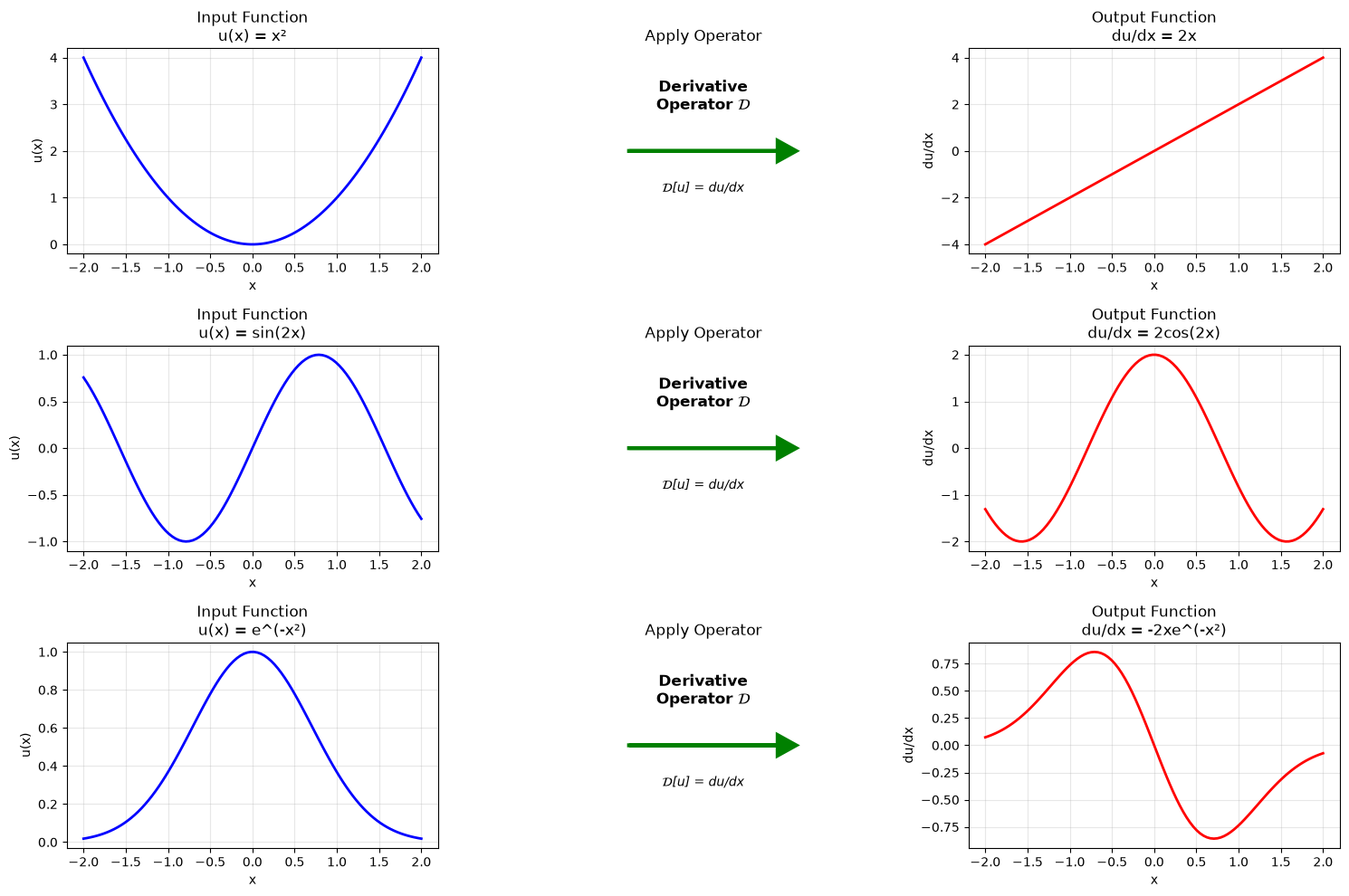
Key Insight: An operator takes a FUNCTION as input and produces a FUNCTION as output!
This is fundamentally different from traditional function approximation.
The Universal Approximation Theorem for Operators#
The Breakthrough Theorem#
Just as the Universal Approximation Theorem tells us neural networks can approximate functions, there’s a remarkable extension:
Theorem (Chen & Chen, 1995): Neural networks can approximate operators that map functions to functions!
Mathematical Statement: For any continuous operator \(\mathcal{G}: V \subset C(K_1) \rightarrow C(K_2)\) and \(\epsilon > 0\), there exist constants such that:
Decoding the Theorem#
This looks complex, but the insight is beautiful:
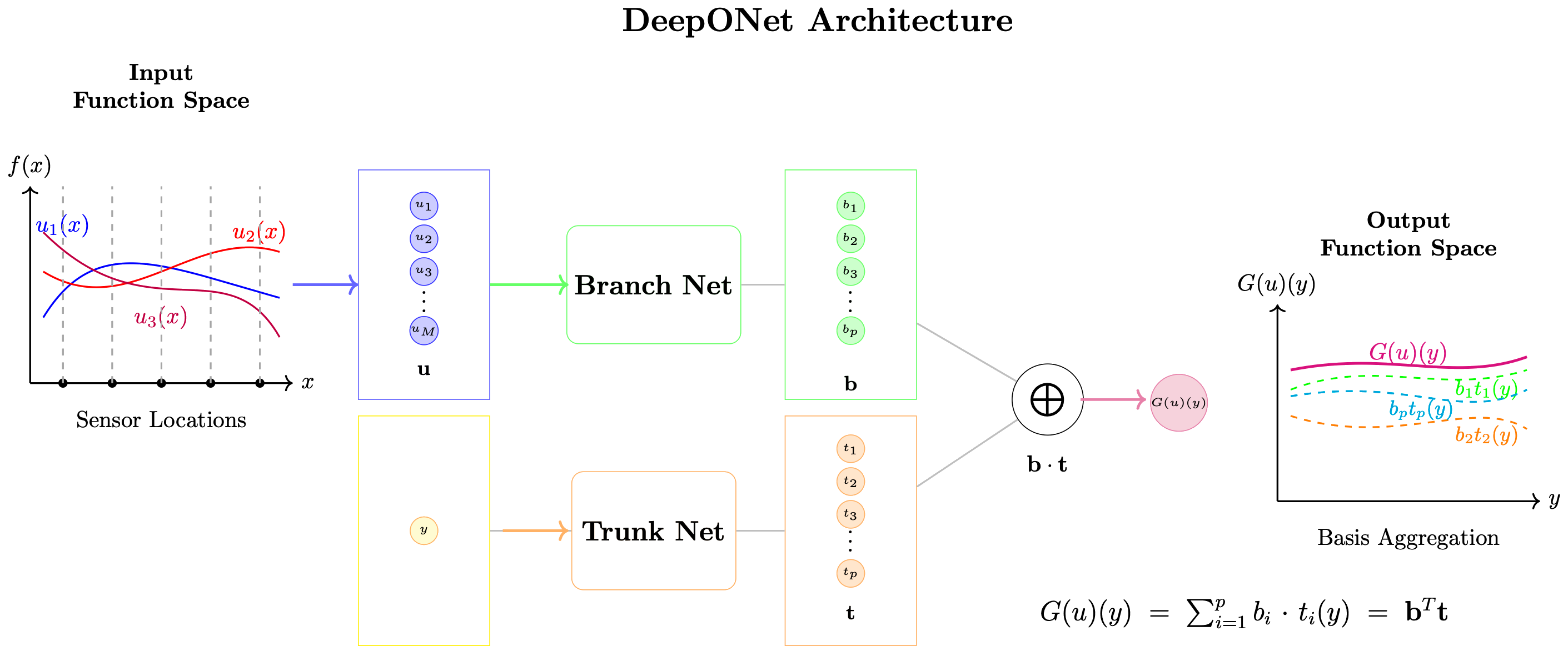
Branch Network: Processes function \(u\) sampled at sensor points \(\{x_j\}\)
Trunk Network: Processes output coordinates \(y\)
Combination: Multiply branch and trunk outputs, then sum
Key insight: Any operator can be written as: $\(\mathcal{G}(u)(y) \approx \sum_{k=1}^p b_k(u) \cdot t_k(y)\)$
where \(b_k\) depends only on the input function and \(t_k\) depends only on the output location!
Visualizing the Operator UAT Structure#
DeepONet Architecture#
DeepONet (Deep Operator Network) is the practical implementation of the Operator Universal Approximation Theorem.
Core Architecture#
where:
Branch network: \(b_k(u) = \mathcal{B}_k([u(x_1), u(x_2), \ldots, u(x_m)])\)
Trunk network: \(t_k(y) = \mathcal{T}_k(y)\)
\(p\): Number of basis functions (typically 50-200)
\(b_0\): Bias term
Training Data Structure#
Input-output pairs: \((u^{(i)}, y^{(j)}, \mathcal{G}(u^{(i)})(y^{(j)}))\)
\(N\) input functions: \(\{u^{(i)}\}_{i=1}^N\)
Each function sampled at \(m\) sensors: \(\{u^{(i)}(x_j)\}_{j=1}^m\)
Corresponding outputs at query points: \(\{\mathcal{G}(u^{(i)})(y_k)\}\)
Loss Function#
Key Advantages#
Resolution independence: Train on one grid, evaluate on any grid
Fast evaluation: Once trained, instant prediction (no iterative solving)
Generalization: Works for new functions not seen during training
Physical consistency: Learns the underlying operator
A function space is a Hilbert space#
Before mapping between function spaces, fix what a function is in this picture.
Choose a basis \(\{\varphi_1,\dots,\varphi_p\}\) and any function in its span is a list of coefficients:
So a function is a vector, the basis functions are the axes, and the coefficients are its coordinates. The inner product \(\langle u,v\rangle=\int u v\,dx\) makes this a Hilbert space, which is what lets us talk about lengths, angles and projections between functions at all.
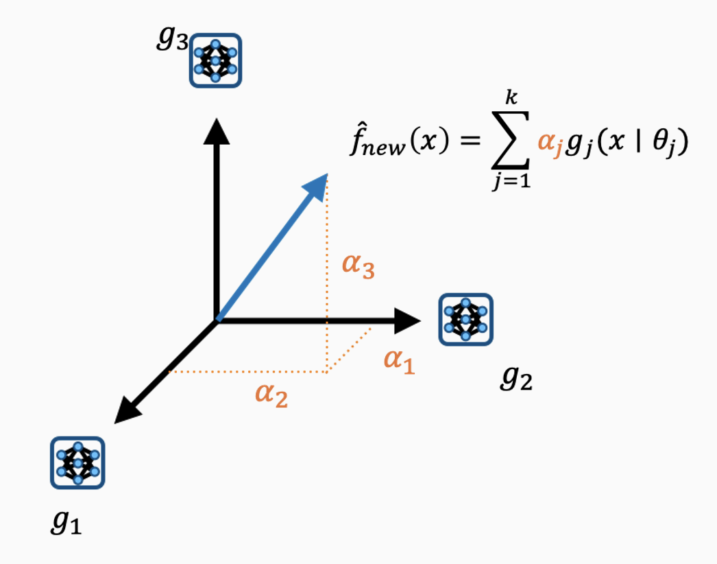
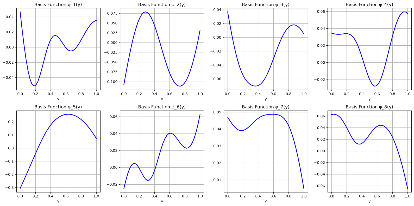
Each axis above is a learned basis function — a small network — and the vector is one function expressed in that basis. An operator then becomes a map from one coefficient vector to another.
Hold onto this: the DeepONet’s trunk network learns those axes, and its branch network produces the coordinates. The final section extracts the learned basis so you can look at the axes it chose.
The 1D Nonlinear Darcy Problem#
Now for something more challenging: A real PDE with nonlinear physics!
Problem Formulation#
The 1D nonlinear Darcy equation models groundwater flow with solution-dependent permeability:
where:
u(x)is the solution field (e.g., pressure or hydraulic head).The \(\kappa(u)\): is non-linear solution-dependent permeability is
κ(u(x)) = 0.2 + u^2(x).The input term
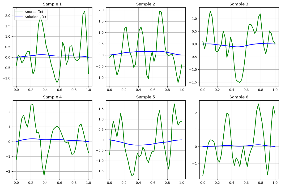
f(x)is a Gaussian random field defined asf(x) ~ GP(0, k(x, x'))such thatk(x, x') = σ^2 exp(-||x - x'||^2 / (2ℓ_x^2)), whereℓ_x = 0.04andσ^2 = 1.0.Homogeneous Dirichlet boundary conditions
u(0) = 0andu(1) = 0are considered at the domain boundaries.
The Operator Learning Challenge#
Goal: Learn the solution operator \(\mathcal{G}\) such that: $\(\mathcal{G}[f] = u\)$
where \(u\) is the solution to the nonlinear Darcy equation for source \(f\).
Key insight: This is much harder than the derivative operator because:
Nonlinear PDE: No analytical solution
Random sources: Infinite variety of input functions
Complex physics: Solution depends on entire source profile
Why This Matters#
Traditional approach: For each new source \(f\), solve the PDE numerically (expensive!)
DeepONet approach: Learn the operator once, then instant evaluation for any new source
Let’s examine the existing Darcy implementation#
import torch
import torch.nn as nn
import torch.optim as optim
import torch.nn.functional as F
import numpy as np
import matplotlib.pyplot as plt
from scipy.sparse import diags
from scipy.sparse.linalg import spsolve
from scipy.stats import multivariate_normal
from tqdm import tqdm

# ========================= CELL 1: Data Generation =========================
def generate_darcy_data(n_funcs=1000, n_points=40):
    """Generate 1D nonlinear Darcy flow data"""

    def permeability(s):
        return 0.2 + s**2

    # Gaussian process for source function
    x = np.linspace(0, 1, n_points)
    l, sigma = 0.04, 1.0
    K = sigma**2 * np.exp(-0.5 * (x[:, None] - x[None, :])**2 / l**2)
    K += 1e-6 * np.eye(n_points)

    def solve_darcy(u_func):
        dx = x[1] - x[0]
        s = np.zeros(n_points)

        for _ in range(100):  # Fixed point iteration
            kappa = permeability(s)
            main_diag = (kappa[1:] + kappa[:-1]) / dx**2
            upper_diag = -kappa[1:-1] / dx**2
            lower_diag = -kappa[1:-1] / dx**2

            A = diags([lower_diag, main_diag, upper_diag], [-1, 0, 1],
                     shape=(n_points-2, n_points-2))

            s_interior = spsolve(A, u_func[1:-1])
            s_new = np.zeros(n_points)
            s_new[1:-1] = s_interior
            s = 0.5 * s_new + 0.5 * s

        return s

    # Generate dataset
    np.random.seed(42)
    X, U, S = [], [], []

    print("Generating Darcy flow dataset...")
    for i in tqdm(range(n_funcs), desc="Solving PDEs"):
        u = multivariate_normal.rvs(mean=np.zeros(n_points), cov=K)
        s = solve_darcy(u)
        X.append(x)
        U.append(u)
        S.append(s)

    X = torch.tensor(np.array(X), dtype=torch.float32)
    U = torch.tensor(np.array(U), dtype=torch.float32)
    S = torch.tensor(np.array(S), dtype=torch.float32)

    print(f"Dataset generated: {n_funcs} functions, {n_points} points each")
    print(f"Input shape: {U.shape}, Output shape: {S.shape}")

    return X, U, S


print("=== DATA GENERATION ===")
X, U, S = generate_darcy_data(n_funcs=1000, n_points=40)

# Plot samples
fig, axes = plt.subplots(2, 3, figsize=(12, 8))
for i in range(6):
    ax = axes[i//3, i%3]
    ax.plot(X[i], U[i], 'g-', label='Source f(x)', linewidth=2)
    ax.plot(X[i], S[i], 'b-', label='Solution u(x)', linewidth=2)
    ax.set_title(f'Sample {i+1}')
    ax.grid(True)
    if i == 0:
        ax.legend()
plt.tight_layout()
plt.savefig('darcy_samples.png', dpi=150)
plt.show()
=== DATA GENERATION ===
Generating Darcy flow dataset...
Solving PDEs: 0%| | 0/1000 [00:00<?, ?it/s]
Solving PDEs: 1%|▏ | 13/1000 [00:00<00:08, 122.59it/s]
Solving PDEs: 3%|▎ | 27/1000 [00:00<00:07, 126.98it/s]
Solving PDEs: 4%|▍ | 40/1000 [00:00<00:07, 128.02it/s]
Solving PDEs: 5%|▌ | 53/1000 [00:00<00:07, 128.78it/s]
Solving PDEs: 7%|▋ | 67/1000 [00:00<00:07, 129.24it/s]
Solving PDEs: 8%|▊ | 80/1000 [00:00<00:07, 129.39it/s]
Solving PDEs: 9%|▉ | 94/1000 [00:00<00:06, 129.84it/s]
Solving PDEs: 11%|█ | 107/1000 [00:00<00:06, 129.84it/s]
Solving PDEs: 12%|█▏ | 121/1000 [00:00<00:06, 130.07it/s]
Solving PDEs: 14%|█▎ | 135/1000 [00:01<00:06, 130.06it/s]
Solving PDEs: 15%|█▍ | 149/1000 [00:01<00:06, 130.14it/s]
Solving PDEs: 16%|█▋ | 163/1000 [00:01<00:06, 130.31it/s]
Solving PDEs: 18%|█▊ | 177/1000 [00:01<00:06, 130.12it/s]
Solving PDEs: 19%|█▉ | 191/1000 [00:01<00:06, 130.29it/s]
Solving PDEs: 20%|██ | 205/1000 [00:01<00:06, 129.94it/s]
Solving PDEs: 22%|██▏ | 219/1000 [00:01<00:06, 129.97it/s]
Solving PDEs: 23%|██▎ | 233/1000 [00:01<00:05, 130.11it/s]
Solving PDEs: 25%|██▍ | 247/1000 [00:01<00:05, 130.13it/s]
Solving PDEs: 26%|██▌ | 261/1000 [00:02<00:05, 130.15it/s]
Solving PDEs: 28%|██▊ | 275/1000 [00:02<00:05, 130.20it/s]
Solving PDEs: 29%|██▉ | 289/1000 [00:02<00:05, 127.50it/s]
Solving PDEs: 30%|███ | 302/1000 [00:02<00:05, 125.33it/s]
Solving PDEs: 32%|███▏ | 315/1000 [00:02<00:05, 125.54it/s]
Solving PDEs: 33%|███▎ | 328/1000 [00:02<00:05, 125.72it/s]
Solving PDEs: 34%|███▍ | 341/1000 [00:02<00:05, 126.69it/s]
Solving PDEs: 35%|███▌ | 354/1000 [00:02<00:05, 127.16it/s]
Solving PDEs: 37%|███▋ | 367/1000 [00:02<00:04, 127.51it/s]
Solving PDEs: 38%|███▊ | 380/1000 [00:02<00:04, 128.19it/s]
Solving PDEs: 39%|███▉ | 394/1000 [00:03<00:04, 128.76it/s]
Solving PDEs: 41%|████ | 408/1000 [00:03<00:04, 129.30it/s]
Solving PDEs: 42%|████▏ | 421/1000 [00:03<00:04, 128.14it/s]
Solving PDEs: 43%|████▎ | 434/1000 [00:03<00:04, 128.42it/s]
Solving PDEs: 45%|████▍ | 447/1000 [00:03<00:04, 128.34it/s]
Solving PDEs: 46%|████▌ | 460/1000 [00:03<00:04, 128.54it/s]
Solving PDEs: 47%|████▋ | 473/1000 [00:03<00:04, 128.53it/s]
Solving PDEs: 49%|████▊ | 486/1000 [00:03<00:03, 128.75it/s]
Solving PDEs: 50%|█████ | 500/1000 [00:03<00:03, 129.25it/s]
Solving PDEs: 51%|█████▏ | 513/1000 [00:03<00:03, 129.14it/s]
Solving PDEs: 53%|█████▎ | 526/1000 [00:04<00:03, 129.35it/s]
Solving PDEs: 54%|█████▍ | 540/1000 [00:04<00:03, 129.59it/s]
Solving PDEs: 55%|█████▌ | 553/1000 [00:04<00:03, 128.48it/s]
Solving PDEs: 57%|█████▋ | 566/1000 [00:04<00:03, 128.10it/s]
Solving PDEs: 58%|█████▊ | 579/1000 [00:04<00:03, 128.28it/s]
Solving PDEs: 59%|█████▉ | 592/1000 [00:04<00:03, 128.64it/s]
Solving PDEs: 60%|██████ | 605/1000 [00:04<00:03, 128.53it/s]
Solving PDEs: 62%|██████▏ | 618/1000 [00:04<00:02, 128.60it/s]
Solving PDEs: 63%|██████▎ | 631/1000 [00:04<00:02, 128.80it/s]
Solving PDEs: 64%|██████▍ | 644/1000 [00:05<00:02, 129.04it/s]
Solving PDEs: 66%|██████▌ | 657/1000 [00:05<00:02, 129.08it/s]
Solving PDEs: 67%|██████▋ | 670/1000 [00:05<00:02, 129.25it/s]
Solving PDEs: 68%|██████▊ | 684/1000 [00:05<00:02, 129.49it/s]
Solving PDEs: 70%|██████▉ | 697/1000 [00:05<00:02, 129.56it/s]
Solving PDEs: 71%|███████ | 710/1000 [00:05<00:02, 129.57it/s]
Solving PDEs: 72%|███████▏ | 724/1000 [00:05<00:02, 129.83it/s]
Solving PDEs: 74%|███████▍ | 738/1000 [00:05<00:02, 129.89it/s]
Solving PDEs: 75%|███████▌ | 751/1000 [00:05<00:01, 129.62it/s]
Solving PDEs: 76%|███████▋ | 765/1000 [00:05<00:01, 129.76it/s]
Solving PDEs: 78%|███████▊ | 779/1000 [00:06<00:01, 129.88it/s]
Solving PDEs: 79%|███████▉ | 792/1000 [00:06<00:01, 129.91it/s]
Solving PDEs: 80%|████████ | 805/1000 [00:06<00:01, 127.76it/s]
Solving PDEs: 82%|████████▏ | 818/1000 [00:06<00:01, 127.94it/s]
Solving PDEs: 83%|████████▎ | 831/1000 [00:06<00:01, 128.50it/s]
Solving PDEs: 84%|████████▍ | 844/1000 [00:06<00:01, 128.84it/s]
Solving PDEs: 86%|████████▌ | 858/1000 [00:06<00:01, 129.38it/s]
Solving PDEs: 87%|████████▋ | 871/1000 [00:06<00:00, 129.46it/s]
Solving PDEs: 88%|████████▊ | 884/1000 [00:06<00:00, 127.63it/s]
Solving PDEs: 90%|████████▉ | 897/1000 [00:06<00:00, 128.10it/s]
Solving PDEs: 91%|█████████ | 910/1000 [00:07<00:00, 128.48it/s]
Solving PDEs: 92%|█████████▏| 923/1000 [00:07<00:00, 128.90it/s]
Solving PDEs: 94%|█████████▎| 936/1000 [00:07<00:00, 129.08it/s]
Solving PDEs: 95%|█████████▍| 949/1000 [00:07<00:00, 128.96it/s]
Solving PDEs: 96%|█████████▌| 962/1000 [00:07<00:00, 129.23it/s]
Solving PDEs: 98%|█████████▊| 975/1000 [00:07<00:00, 129.38it/s]
Solving PDEs: 99%|█████████▉| 988/1000 [00:07<00:00, 129.41it/s]
Solving PDEs: 100%|██████████| 1000/1000 [00:07<00:00, 128.89it/s]
Dataset generated: 1000 functions, 40 points each
Input shape: torch.Size([1000, 40]), Output shape: torch.Size([1000, 40])
DeepONet Architecture#
class DeepONet(nn.Module):
    def __init__(self, branch_dim, trunk_dim, p_dim=128, hidden_dim=256):
        super().__init__()

        # Branch network (processes input function)
        self.branch = nn.Sequential(
            nn.Linear(branch_dim, hidden_dim),
            nn.GELU(),
            nn.Linear(hidden_dim, hidden_dim),
            nn.GELU(),
            nn.Linear(hidden_dim, p_dim)
        )

        # Trunk network (processes query points)
        self.trunk = nn.Sequential(
            nn.Linear(trunk_dim, hidden_dim),
            nn.GELU(),
            nn.Linear(hidden_dim, hidden_dim),
            nn.GELU(),
            nn.Linear(hidden_dim, p_dim)
        )

    def forward(self, u_vals, y_locs):
        branch_out = self.branch(u_vals)  # [batch, p_dim]
        trunk_out = self.trunk(y_locs)    # [batch, n_points, p_dim]

        # Dot product: sum over p_dim
        return torch.einsum('bp,bnp->bn', branch_out, trunk_out)


print("\n=== DEEPONET ARCHITECTURE ===")
print(f"Using device: {device}")

model = DeepONet(branch_dim=U.shape[1], trunk_dim=1, p_dim=128).to(device)

# Print model info
total_params = sum(p.numel() for p in model.parameters())
trainable_params = sum(p.numel() for p in model.parameters() if p.requires_grad)

print(f"Total parameters: {total_params:,}")
print(f"Trainable parameters: {trainable_params:,}")
=== DEEPONET ARCHITECTURE ===
Using device: mps
Total parameters: 208,384
Trainable parameters: 208,384
Training#
def setup_training(X, U, S, model, device):
    """Prepare data and optimizer for training"""
    # Split data
    n_train = int(0.8 * len(U))
    U_train, S_train = U[:n_train].to(device), S[:n_train].to(device)
    U_test, S_test = U[n_train:].to(device), S[n_train:].to(device)
    X_train, X_test = X[:n_train].to(device), X[n_train:].to(device)

    # Normalize targets
    S_mean, S_std = S_train.mean(), S_train.std()
    S_train_norm = (S_train - S_mean) / S_std
    S_test_norm = (S_test - S_mean) / S_std

    print(f"Training samples: {len(U_train)}")
    print(f"Test samples: {len(U_test)}")
    print(f"Target normalization - Mean: {S_mean:.4f}, Std: {S_std:.4f}")

    return (U_train, S_train_norm, X_train, U_test, S_test_norm, X_test, S_mean, S_std)

def train_model(model, train_data, epochs=5000, batch_size=64, lr=1e-3):
    """Train the DeepONet model"""
    U_train, S_train_norm, X_train, _, _, _, _, _ = train_data

    optimizer = optim.Adam(model.parameters(), lr=lr, weight_decay=1e-5)
    scheduler = optim.lr_scheduler.CosineAnnealingLR(optimizer, T_max=epochs)

    print(f"Starting training: {epochs} epochs, batch size {batch_size}, lr {lr}")

    model.train()
    losses = []

    pbar = tqdm(range(epochs), desc="Training")
    for epoch in pbar:
        # Random batch
        idx = torch.randperm(len(U_train))[:batch_size]
        u_batch = U_train[idx]
        s_batch = S_train_norm[idx]
        x_batch = X_train[idx].unsqueeze(-1)  # [batch, n_points, 1]

        # Forward pass
        s_pred = model(u_batch, x_batch)
        loss = F.mse_loss(s_pred, s_batch)

        # Backward pass
        optimizer.zero_grad()
        loss.backward()
        optimizer.step()
        scheduler.step()

        losses.append(loss.item())

        if epoch % 100 == 0:
            pbar.set_postfix({
                'Loss': f'{loss.item():.6f}',
                'LR': f'{scheduler.get_last_lr()[0]:.2e}'
            })

    print("Training completed!")
    return losses


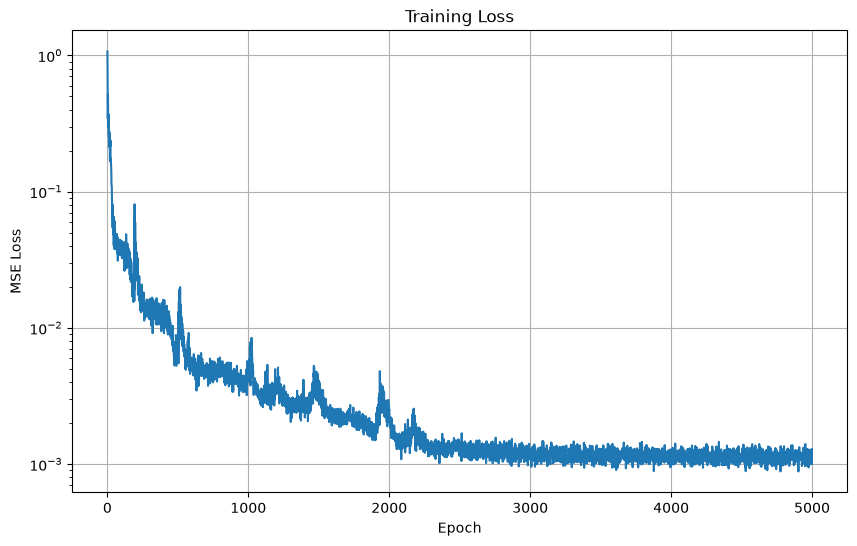
print("\n=== TRAINING ===")
train_data = setup_training(X, U, S, model, device)
losses = train_model(model, train_data, epochs=5000)

# Plot training loss
plt.figure(figsize=(10, 6))
plt.plot(losses)
plt.title('Training Loss')
plt.xlabel('Epoch')
plt.ylabel('MSE Loss')
plt.yscale('log')
plt.grid(True)
plt.savefig('training_loss.png', dpi=150)
plt.show()
=== TRAINING ===
Training samples: 800
Test samples: 200
Target normalization - Mean: -0.0046, Std: 0.1468
Starting training: 5000 epochs, batch size 64, lr 0.001
Training: 0%| | 0/5000 [00:00<?, ?it/s]
Training: 0%| | 0/5000 [00:00<?, ?it/s, Loss=1.067647, LR=1.00e-03]
Training: 0%| | 8/5000 [00:00<01:03, 79.08it/s, Loss=1.067647, LR=1.00e-03]
Training: 1%| | 44/5000 [00:00<00:20, 242.33it/s, Loss=1.067647, LR=1.00e-03]
Training: 2%|▏ | 83/5000 [00:00<00:15, 308.37it/s, Loss=1.067647, LR=1.00e-03]
Training: 2%|▏ | 83/5000 [00:00<00:15, 308.37it/s, Loss=0.043588, LR=9.99e-04]
Training: 2%|▏ | 124/5000 [00:00<00:14, 345.73it/s, Loss=0.043588, LR=9.99e-04]
Training: 3%|▎ | 164/5000 [00:00<00:13, 362.07it/s, Loss=0.043588, LR=9.99e-04]
Training: 3%|▎ | 164/5000 [00:00<00:13, 362.07it/s, Loss=0.042418, LR=9.96e-04]
Training: 4%|▍ | 201/5000 [00:00<00:13, 361.53it/s, Loss=0.042418, LR=9.96e-04]
Training: 5%|▍ | 238/5000 [00:00<00:14, 332.29it/s, Loss=0.042418, LR=9.96e-04]
Training: 5%|▌ | 272/5000 [00:00<00:15, 312.15it/s, Loss=0.042418, LR=9.96e-04]
Training: 5%|▌ | 272/5000 [00:00<00:15, 312.15it/s, Loss=0.013238, LR=9.91e-04]
Training: 6%|▌ | 304/5000 [00:00<00:15, 296.05it/s, Loss=0.013238, LR=9.91e-04]
Training: 7%|▋ | 334/5000 [00:01<00:16, 283.57it/s, Loss=0.013238, LR=9.91e-04]
Training: 7%|▋ | 363/5000 [00:01<00:17, 268.97it/s, Loss=0.013238, LR=9.91e-04]
Training: 8%|▊ | 391/5000 [00:01<00:18, 245.58it/s, Loss=0.013238, LR=9.91e-04]
Training: 8%|▊ | 391/5000 [00:01<00:18, 245.58it/s, Loss=0.012250, LR=9.84e-04]
Training: 8%|▊ | 416/5000 [00:01<00:21, 217.40it/s, Loss=0.012250, LR=9.84e-04]
Training: 9%|▉ | 439/5000 [00:01<00:21, 210.83it/s, Loss=0.012250, LR=9.84e-04]
Training: 9%|▉ | 461/5000 [00:01<00:23, 195.53it/s, Loss=0.012250, LR=9.84e-04]
Training: 10%|▉ | 481/5000 [00:01<00:24, 187.17it/s, Loss=0.012250, LR=9.84e-04]
Training: 10%|█ | 500/5000 [00:02<00:24, 182.87it/s, Loss=0.012250, LR=9.84e-04]
Training: 10%|█ | 500/5000 [00:02<00:24, 182.87it/s, Loss=0.006737, LR=9.75e-04]
Training: 10%|█ | 519/5000 [00:02<00:25, 177.76it/s, Loss=0.006737, LR=9.75e-04]
Training: 11%|█ | 537/5000 [00:02<00:25, 174.91it/s, Loss=0.006737, LR=9.75e-04]
Training: 11%|█ | 555/5000 [00:02<00:25, 173.81it/s, Loss=0.006737, LR=9.75e-04]
Training: 11%|█▏ | 573/5000 [00:02<00:26, 168.43it/s, Loss=0.006737, LR=9.75e-04]
Training: 12%|█▏ | 590/5000 [00:02<00:26, 167.42it/s, Loss=0.006737, LR=9.75e-04]
Training: 12%|█▏ | 590/5000 [00:02<00:26, 167.42it/s, Loss=0.005233, LR=9.65e-04]
Training: 12%|█▏ | 607/5000 [00:02<00:26, 166.18it/s, Loss=0.005233, LR=9.65e-04]
Training: 13%|█▎ | 627/5000 [00:02<00:25, 174.83it/s, Loss=0.005233, LR=9.65e-04]
Training: 13%|█▎ | 645/5000 [00:02<00:24, 175.68it/s, Loss=0.005233, LR=9.65e-04]
Training: 14%|█▎ | 675/5000 [00:02<00:20, 210.54it/s, Loss=0.005233, LR=9.65e-04]
Training: 14%|█▎ | 675/5000 [00:03<00:20, 210.54it/s, Loss=0.004874, LR=9.52e-04]
Training: 14%|█▍ | 707/5000 [00:03<00:17, 240.25it/s, Loss=0.004874, LR=9.52e-04]
Training: 15%|█▍ | 745/5000 [00:03<00:15, 280.03it/s, Loss=0.004874, LR=9.52e-04]
Training: 16%|█▌ | 782/5000 [00:03<00:13, 304.89it/s, Loss=0.004874, LR=9.52e-04]
Training: 16%|█▌ | 782/5000 [00:03<00:13, 304.89it/s, Loss=0.005182, LR=9.38e-04]
Training: 16%|█▋ | 813/5000 [00:03<00:14, 298.13it/s, Loss=0.005182, LR=9.38e-04]
Training: 17%|█▋ | 843/5000 [00:03<00:14, 288.56it/s, Loss=0.005182, LR=9.38e-04]
Training: 17%|█▋ | 872/5000 [00:03<00:14, 282.26it/s, Loss=0.005182, LR=9.38e-04]
Training: 17%|█▋ | 872/5000 [00:03<00:14, 282.26it/s, Loss=0.004325, LR=9.22e-04]
Training: 18%|█▊ | 901/5000 [00:03<00:14, 276.28it/s, Loss=0.004325, LR=9.22e-04]
Training: 19%|█▊ | 929/5000 [00:03<00:14, 271.53it/s, Loss=0.004325, LR=9.22e-04]
Training: 19%|█▉ | 957/5000 [00:03<00:15, 268.08it/s, Loss=0.004325, LR=9.22e-04]
Training: 20%|█▉ | 984/5000 [00:04<00:14, 268.17it/s, Loss=0.004325, LR=9.22e-04]
Training: 20%|█▉ | 984/5000 [00:04<00:14, 268.17it/s, Loss=0.004391, LR=9.04e-04]
Training: 20%|██ | 1011/5000 [00:04<00:15, 265.67it/s, Loss=0.004391, LR=9.04e-04]
Training: 21%|██ | 1038/5000 [00:04<00:14, 264.37it/s, Loss=0.004391, LR=9.04e-04]
Training: 21%|██▏ | 1065/5000 [00:04<00:14, 263.12it/s, Loss=0.004391, LR=9.04e-04]
Training: 22%|██▏ | 1092/5000 [00:04<00:14, 261.28it/s, Loss=0.004391, LR=9.04e-04]
Training: 22%|██▏ | 1092/5000 [00:04<00:14, 261.28it/s, Loss=0.003387, LR=8.85e-04]
Training: 22%|██▏ | 1119/5000 [00:04<00:14, 261.26it/s, Loss=0.003387, LR=8.85e-04]
Training: 23%|██▎ | 1146/5000 [00:04<00:14, 262.94it/s, Loss=0.003387, LR=8.85e-04]
Training: 23%|██▎ | 1173/5000 [00:04<00:14, 262.85it/s, Loss=0.003387, LR=8.85e-04]
Training: 24%|██▍ | 1200/5000 [00:04<00:14, 263.93it/s, Loss=0.003387, LR=8.85e-04]
Training: 24%|██▍ | 1200/5000 [00:04<00:14, 263.93it/s, Loss=0.004022, LR=8.64e-04]
Training: 25%|██▍ | 1227/5000 [00:04<00:14, 262.64it/s, Loss=0.004022, LR=8.64e-04]
Training: 25%|██▌ | 1254/5000 [00:05<00:14, 262.17it/s, Loss=0.004022, LR=8.64e-04]
Training: 26%|██▌ | 1281/5000 [00:05<00:14, 260.27it/s, Loss=0.004022, LR=8.64e-04]
Training: 26%|██▌ | 1281/5000 [00:05<00:14, 260.27it/s, Loss=0.002578, LR=8.42e-04]
Training: 26%|██▌ | 1308/5000 [00:05<00:14, 259.61it/s, Loss=0.002578, LR=8.42e-04]
Training: 27%|██▋ | 1334/5000 [00:05<00:14, 259.02it/s, Loss=0.002578, LR=8.42e-04]
Training: 27%|██▋ | 1360/5000 [00:05<00:14, 258.38it/s, Loss=0.002578, LR=8.42e-04]
Training: 28%|██▊ | 1386/5000 [00:05<00:13, 258.39it/s, Loss=0.002578, LR=8.42e-04]
Training: 28%|██▊ | 1386/5000 [00:05<00:13, 258.39it/s, Loss=0.002691, LR=8.18e-04]
Training: 28%|██▊ | 1413/5000 [00:05<00:13, 260.63it/s, Loss=0.002691, LR=8.18e-04]
Training: 29%|██▉ | 1440/5000 [00:05<00:13, 260.95it/s, Loss=0.002691, LR=8.18e-04]
Training: 29%|██▉ | 1467/5000 [00:05<00:13, 260.76it/s, Loss=0.002691, LR=8.18e-04]
Training: 30%|██▉ | 1494/5000 [00:05<00:13, 260.48it/s, Loss=0.002691, LR=8.18e-04]
Training: 30%|██▉ | 1494/5000 [00:06<00:13, 260.48it/s, Loss=0.002897, LR=7.94e-04]
Training: 30%|███ | 1521/5000 [00:06<00:13, 259.96it/s, Loss=0.002897, LR=7.94e-04]
Training: 31%|███ | 1548/5000 [00:06<00:13, 260.05it/s, Loss=0.002897, LR=7.94e-04]
Training: 32%|███▏ | 1575/5000 [00:06<00:13, 259.42it/s, Loss=0.002897, LR=7.94e-04]
Training: 32%|███▏ | 1575/5000 [00:06<00:13, 259.42it/s, Loss=0.002324, LR=7.68e-04]
Training: 32%|███▏ | 1601/5000 [00:06<00:13, 259.05it/s, Loss=0.002324, LR=7.68e-04]
Training: 33%|███▎ | 1627/5000 [00:06<00:13, 259.28it/s, Loss=0.002324, LR=7.68e-04]
Training: 33%|███▎ | 1654/5000 [00:06<00:12, 259.87it/s, Loss=0.002324, LR=7.68e-04]
Training: 34%|███▎ | 1680/5000 [00:06<00:12, 259.50it/s, Loss=0.002324, LR=7.68e-04]
Training: 34%|███▎ | 1680/5000 [00:06<00:12, 259.50it/s, Loss=0.002133, LR=7.41e-04]
Training: 34%|███▍ | 1706/5000 [00:06<00:12, 259.08it/s, Loss=0.002133, LR=7.41e-04]
Training: 35%|███▍ | 1732/5000 [00:06<00:12, 258.78it/s, Loss=0.002133, LR=7.41e-04]
Training: 35%|███▌ | 1759/5000 [00:07<00:12, 259.37it/s, Loss=0.002133, LR=7.41e-04]
Training: 36%|███▌ | 1786/5000 [00:07<00:12, 260.80it/s, Loss=0.002133, LR=7.41e-04]
Training: 36%|███▌ | 1786/5000 [00:07<00:12, 260.80it/s, Loss=0.001840, LR=7.13e-04]
Training: 36%|███▋ | 1813/5000 [00:07<00:12, 260.18it/s, Loss=0.001840, LR=7.13e-04]
Training: 37%|███▋ | 1840/5000 [00:07<00:12, 259.79it/s, Loss=0.001840, LR=7.13e-04]
Training: 37%|███▋ | 1866/5000 [00:07<00:12, 259.34it/s, Loss=0.001840, LR=7.13e-04]
Training: 38%|███▊ | 1892/5000 [00:07<00:12, 257.60it/s, Loss=0.001840, LR=7.13e-04]
Training: 38%|███▊ | 1892/5000 [00:07<00:12, 257.60it/s, Loss=0.001498, LR=6.84e-04]
Training: 38%|███▊ | 1918/5000 [00:07<00:11, 257.03it/s, Loss=0.001498, LR=6.84e-04]
Training: 39%|███▉ | 1945/5000 [00:07<00:11, 259.26it/s, Loss=0.001498, LR=6.84e-04]
Training: 39%|███▉ | 1971/5000 [00:07<00:11, 258.24it/s, Loss=0.001498, LR=6.84e-04]
Training: 40%|███▉ | 1997/5000 [00:07<00:11, 257.82it/s, Loss=0.001498, LR=6.84e-04]
Training: 40%|███▉ | 1997/5000 [00:07<00:11, 257.82it/s, Loss=0.002506, LR=6.54e-04]
Training: 40%|████ | 2023/5000 [00:08<00:11, 257.58it/s, Loss=0.002506, LR=6.54e-04]
Training: 41%|████ | 2051/5000 [00:08<00:11, 261.46it/s, Loss=0.002506, LR=6.54e-04]
Training: 42%|████▏ | 2078/5000 [00:08<00:11, 260.68it/s, Loss=0.002506, LR=6.54e-04]
Training: 42%|████▏ | 2078/5000 [00:08<00:11, 260.68it/s, Loss=0.001507, LR=6.24e-04]
Training: 42%|████▏ | 2105/5000 [00:08<00:11, 260.91it/s, Loss=0.001507, LR=6.24e-04]
Training: 43%|████▎ | 2132/5000 [00:08<00:11, 260.12it/s, Loss=0.001507, LR=6.24e-04]
Training: 43%|████▎ | 2159/5000 [00:08<00:11, 258.19it/s, Loss=0.001507, LR=6.24e-04]
Training: 44%|████▎ | 2185/5000 [00:08<00:10, 257.83it/s, Loss=0.001507, LR=6.24e-04]
Training: 44%|████▎ | 2185/5000 [00:08<00:10, 257.83it/s, Loss=0.001777, LR=5.93e-04]
Training: 44%|████▍ | 2211/5000 [00:08<00:10, 257.07it/s, Loss=0.001777, LR=5.93e-04]
Training: 45%|████▍ | 2238/5000 [00:08<00:10, 258.99it/s, Loss=0.001777, LR=5.93e-04]
Training: 45%|████▌ | 2265/5000 [00:08<00:10, 260.34it/s, Loss=0.001777, LR=5.93e-04]
Training: 46%|████▌ | 2292/5000 [00:09<00:10, 261.66it/s, Loss=0.001777, LR=5.93e-04]
Training: 46%|████▌ | 2292/5000 [00:09<00:10, 261.66it/s, Loss=0.001261, LR=5.62e-04]
Training: 46%|████▋ | 2319/5000 [00:09<00:10, 260.75it/s, Loss=0.001261, LR=5.62e-04]
Training: 47%|████▋ | 2346/5000 [00:09<00:10, 260.80it/s, Loss=0.001261, LR=5.62e-04]
Training: 47%|████▋ | 2373/5000 [00:09<00:10, 260.69it/s, Loss=0.001261, LR=5.62e-04]
Training: 48%|████▊ | 2400/5000 [00:09<00:09, 260.05it/s, Loss=0.001261, LR=5.62e-04]
Training: 48%|████▊ | 2400/5000 [00:09<00:09, 260.05it/s, Loss=0.001403, LR=5.31e-04]
Training: 49%|████▊ | 2427/5000 [00:09<00:09, 258.51it/s, Loss=0.001403, LR=5.31e-04]
Training: 49%|████▉ | 2453/5000 [00:09<00:09, 258.47it/s, Loss=0.001403, LR=5.31e-04]
Training: 50%|████▉ | 2480/5000 [00:09<00:09, 260.15it/s, Loss=0.001403, LR=5.31e-04]
Training: 50%|████▉ | 2480/5000 [00:09<00:09, 260.15it/s, Loss=0.001178, LR=5.00e-04]
Training: 50%|█████ | 2507/5000 [00:09<00:09, 259.42it/s, Loss=0.001178, LR=5.00e-04]
Training: 51%|█████ | 2533/5000 [00:09<00:09, 259.44it/s, Loss=0.001178, LR=5.00e-04]
Training: 51%|█████ | 2559/5000 [00:10<00:09, 258.51it/s, Loss=0.001178, LR=5.00e-04]
Training: 52%|█████▏ | 2585/5000 [00:10<00:09, 257.73it/s, Loss=0.001178, LR=5.00e-04]
Training: 52%|█████▏ | 2585/5000 [00:10<00:09, 257.73it/s, Loss=0.001260, LR=4.68e-04]
Training: 52%|█████▏ | 2611/5000 [00:10<00:09, 257.38it/s, Loss=0.001260, LR=4.68e-04]
Training: 53%|█████▎ | 2638/5000 [00:10<00:09, 258.46it/s, Loss=0.001260, LR=4.68e-04]
Training: 53%|█████▎ | 2664/5000 [00:10<00:09, 257.98it/s, Loss=0.001260, LR=4.68e-04]
Training: 54%|█████▍ | 2691/5000 [00:10<00:08, 258.72it/s, Loss=0.001260, LR=4.68e-04]
Training: 54%|█████▍ | 2691/5000 [00:10<00:08, 258.72it/s, Loss=0.001132, LR=4.37e-04]
Training: 54%|█████▍ | 2717/5000 [00:10<00:08, 258.62it/s, Loss=0.001132, LR=4.37e-04]
Training: 55%|█████▍ | 2743/5000 [00:10<00:08, 258.42it/s, Loss=0.001132, LR=4.37e-04]
Training: 55%|█████▌ | 2770/5000 [00:10<00:08, 259.62it/s, Loss=0.001132, LR=4.37e-04]
Training: 56%|█████▌ | 2797/5000 [00:11<00:08, 260.06it/s, Loss=0.001132, LR=4.37e-04]
Training: 56%|█████▌ | 2797/5000 [00:11<00:08, 260.06it/s, Loss=0.001163, LR=4.06e-04]
Training: 56%|█████▋ | 2824/5000 [00:11<00:08, 261.28it/s, Loss=0.001163, LR=4.06e-04]
Training: 57%|█████▋ | 2851/5000 [00:11<00:08, 261.80it/s, Loss=0.001163, LR=4.06e-04]
Training: 58%|█████▊ | 2878/5000 [00:11<00:08, 260.71it/s, Loss=0.001163, LR=4.06e-04]
Training: 58%|█████▊ | 2878/5000 [00:11<00:08, 260.71it/s, Loss=0.001137, LR=3.75e-04]
Training: 58%|█████▊ | 2905/5000 [00:11<00:08, 259.32it/s, Loss=0.001137, LR=3.75e-04]
Training: 59%|█████▊ | 2931/5000 [00:11<00:07, 259.19it/s, Loss=0.001137, LR=3.75e-04]
Training: 59%|█████▉ | 2957/5000 [00:11<00:07, 259.21it/s, Loss=0.001137, LR=3.75e-04]
Training: 60%|█████▉ | 2983/5000 [00:11<00:07, 258.59it/s, Loss=0.001137, LR=3.75e-04]
Training: 60%|█████▉ | 2983/5000 [00:11<00:07, 258.59it/s, Loss=0.001235, LR=3.45e-04]
Training: 60%|██████ | 3010/5000 [00:11<00:07, 260.10it/s, Loss=0.001235, LR=3.45e-04]
Training: 61%|██████ | 3037/5000 [00:11<00:07, 259.46it/s, Loss=0.001235, LR=3.45e-04]
Training: 61%|██████▏ | 3063/5000 [00:12<00:07, 259.49it/s, Loss=0.001235, LR=3.45e-04]
Training: 62%|██████▏ | 3090/5000 [00:12<00:07, 261.36it/s, Loss=0.001235, LR=3.45e-04]
Training: 62%|██████▏ | 3090/5000 [00:12<00:07, 261.36it/s, Loss=0.001108, LR=3.16e-04]
Training: 62%|██████▏ | 3117/5000 [00:12<00:07, 260.90it/s, Loss=0.001108, LR=3.16e-04]
Training: 63%|██████▎ | 3144/5000 [00:12<00:07, 260.18it/s, Loss=0.001108, LR=3.16e-04]
Training: 63%|██████▎ | 3171/5000 [00:12<00:07, 260.41it/s, Loss=0.001108, LR=3.16e-04]
Training: 64%|██████▍ | 3198/5000 [00:12<00:06, 260.91it/s, Loss=0.001108, LR=3.16e-04]
Training: 64%|██████▍ | 3198/5000 [00:12<00:06, 260.91it/s, Loss=0.001140, LR=2.87e-04]
Training: 64%|██████▍ | 3225/5000 [00:12<00:06, 259.31it/s, Loss=0.001140, LR=2.87e-04]
Training: 65%|██████▌ | 3251/5000 [00:12<00:06, 259.29it/s, Loss=0.001140, LR=2.87e-04]
Training: 66%|██████▌ | 3278/5000 [00:12<00:06, 259.68it/s, Loss=0.001140, LR=2.87e-04]
Training: 66%|██████▌ | 3278/5000 [00:12<00:06, 259.68it/s, Loss=0.001131, LR=2.59e-04]
Training: 66%|██████▌ | 3304/5000 [00:12<00:06, 259.45it/s, Loss=0.001131, LR=2.59e-04]
Training: 67%|██████▋ | 3331/5000 [00:13<00:06, 259.64it/s, Loss=0.001131, LR=2.59e-04]
Training: 67%|██████▋ | 3358/5000 [00:13<00:06, 261.41it/s, Loss=0.001131, LR=2.59e-04]
Training: 68%|██████▊ | 3386/5000 [00:13<00:06, 264.75it/s, Loss=0.001131, LR=2.59e-04]
Training: 68%|██████▊ | 3386/5000 [00:13<00:06, 264.75it/s, Loss=0.001011, LR=2.32e-04]
Training: 68%|██████▊ | 3413/5000 [00:13<00:05, 265.08it/s, Loss=0.001011, LR=2.32e-04]
Training: 69%|██████▉ | 3441/5000 [00:13<00:05, 266.64it/s, Loss=0.001011, LR=2.32e-04]
Training: 69%|██████▉ | 3468/5000 [00:13<00:05, 264.24it/s, Loss=0.001011, LR=2.32e-04]
Training: 70%|██████▉ | 3495/5000 [00:13<00:05, 263.24it/s, Loss=0.001011, LR=2.32e-04]
Training: 70%|██████▉ | 3495/5000 [00:13<00:05, 263.24it/s, Loss=0.001295, LR=2.06e-04]
Training: 70%|███████ | 3522/5000 [00:13<00:05, 263.27it/s, Loss=0.001295, LR=2.06e-04]
Training: 71%|███████ | 3549/5000 [00:13<00:05, 263.73it/s, Loss=0.001295, LR=2.06e-04]
Training: 72%|███████▏ | 3576/5000 [00:13<00:05, 262.96it/s, Loss=0.001295, LR=2.06e-04]
Training: 72%|███████▏ | 3576/5000 [00:14<00:05, 262.96it/s, Loss=0.001142, LR=1.81e-04]
Training: 72%|███████▏ | 3603/5000 [00:14<00:05, 261.14it/s, Loss=0.001142, LR=1.81e-04]
Training: 73%|███████▎ | 3630/5000 [00:14<00:05, 261.35it/s, Loss=0.001142, LR=1.81e-04]
Training: 73%|███████▎ | 3657/5000 [00:14<00:05, 261.30it/s, Loss=0.001142, LR=1.81e-04]
Training: 74%|███████▎ | 3684/5000 [00:14<00:05, 260.29it/s, Loss=0.001142, LR=1.81e-04]
Training: 74%|███████▎ | 3684/5000 [00:14<00:05, 260.29it/s, Loss=0.001146, LR=1.57e-04]
Training: 74%|███████▍ | 3711/5000 [00:14<00:04, 259.56it/s, Loss=0.001146, LR=1.57e-04]
Training: 75%|███████▍ | 3737/5000 [00:14<00:04, 259.39it/s, Loss=0.001146, LR=1.57e-04]
Training: 75%|███████▌ | 3764/5000 [00:14<00:04, 260.73it/s, Loss=0.001146, LR=1.57e-04]
Training: 76%|███████▌ | 3791/5000 [00:14<00:04, 262.19it/s, Loss=0.001146, LR=1.57e-04]
Training: 76%|███████▌ | 3791/5000 [00:14<00:04, 262.19it/s, Loss=0.001214, LR=1.35e-04]
Training: 76%|███████▋ | 3818/5000 [00:14<00:04, 260.33it/s, Loss=0.001214, LR=1.35e-04]
Training: 77%|███████▋ | 3845/5000 [00:15<00:04, 261.58it/s, Loss=0.001214, LR=1.35e-04]
Training: 77%|███████▋ | 3872/5000 [00:15<00:04, 262.75it/s, Loss=0.001214, LR=1.35e-04]
Training: 78%|███████▊ | 3899/5000 [00:15<00:04, 260.46it/s, Loss=0.001214, LR=1.35e-04]
Training: 78%|███████▊ | 3899/5000 [00:15<00:04, 260.46it/s, Loss=0.001063, LR=1.15e-04]
Training: 79%|███████▊ | 3926/5000 [00:15<00:04, 261.06it/s, Loss=0.001063, LR=1.15e-04]
Training: 79%|███████▉ | 3953/5000 [00:15<00:04, 260.78it/s, Loss=0.001063, LR=1.15e-04]
Training: 80%|███████▉ | 3980/5000 [00:15<00:03, 260.75it/s, Loss=0.001063, LR=1.15e-04]
Training: 80%|███████▉ | 3980/5000 [00:15<00:03, 260.75it/s, Loss=0.001273, LR=9.53e-05]
Training: 80%|████████ | 4007/5000 [00:15<00:03, 259.97it/s, Loss=0.001273, LR=9.53e-05]
Training: 81%|████████ | 4034/5000 [00:15<00:03, 261.14it/s, Loss=0.001273, LR=9.53e-05]
Training: 81%|████████ | 4061/5000 [00:15<00:03, 243.53it/s, Loss=0.001273, LR=9.53e-05]
Training: 82%|████████▏ | 4086/5000 [00:15<00:03, 242.29it/s, Loss=0.001273, LR=9.53e-05]
Training: 82%|████████▏ | 4086/5000 [00:16<00:03, 242.29it/s, Loss=0.001080, LR=7.77e-05]
Training: 82%|████████▏ | 4120/5000 [00:16<00:03, 268.51it/s, Loss=0.001080, LR=7.77e-05]
Training: 83%|████████▎ | 4151/5000 [00:16<00:03, 280.27it/s, Loss=0.001080, LR=7.77e-05]
Training: 84%|████████▎ | 4187/5000 [00:16<00:02, 302.09it/s, Loss=0.001080, LR=7.77e-05]
Training: 84%|████████▎ | 4187/5000 [00:16<00:02, 302.09it/s, Loss=0.000988, LR=6.17e-05]
Training: 84%|████████▍ | 4221/5000 [00:16<00:02, 310.87it/s, Loss=0.000988, LR=6.17e-05]
Training: 85%|████████▌ | 4253/5000 [00:16<00:02, 295.84it/s, Loss=0.000988, LR=6.17e-05]
Training: 86%|████████▌ | 4283/5000 [00:16<00:02, 282.30it/s, Loss=0.000988, LR=6.17e-05]
Training: 86%|████████▌ | 4283/5000 [00:16<00:02, 282.30it/s, Loss=0.001254, LR=4.75e-05]
Training: 86%|████████▌ | 4312/5000 [00:16<00:02, 265.61it/s, Loss=0.001254, LR=4.75e-05]
Training: 87%|████████▋ | 4339/5000 [00:16<00:02, 247.62it/s, Loss=0.001254, LR=4.75e-05]
Training: 87%|████████▋ | 4365/5000 [00:17<00:02, 229.79it/s, Loss=0.001254, LR=4.75e-05]
Training: 88%|████████▊ | 4389/5000 [00:17<00:02, 220.08it/s, Loss=0.001254, LR=4.75e-05]
Training: 88%|████████▊ | 4389/5000 [00:17<00:02, 220.08it/s, Loss=0.001173, LR=3.50e-05]
Training: 88%|████████▊ | 4412/5000 [00:17<00:02, 204.02it/s, Loss=0.001173, LR=3.50e-05]
Training: 89%|████████▊ | 4433/5000 [00:17<00:02, 198.13it/s, Loss=0.001173, LR=3.50e-05]
Training: 89%|████████▉ | 4456/5000 [00:17<00:02, 205.93it/s, Loss=0.001173, LR=3.50e-05]
Training: 90%|████████▉ | 4479/5000 [00:17<00:02, 211.62it/s, Loss=0.001173, LR=3.50e-05]
Training: 90%|████████▉ | 4479/5000 [00:17<00:02, 211.62it/s, Loss=0.001047, LR=2.44e-05]
Training: 90%|█████████ | 4501/5000 [00:17<00:02, 206.51it/s, Loss=0.001047, LR=2.44e-05]
Training: 90%|█████████ | 4522/5000 [00:17<00:02, 191.15it/s, Loss=0.001047, LR=2.44e-05]
Training: 91%|█████████ | 4543/5000 [00:17<00:02, 195.45it/s, Loss=0.001047, LR=2.44e-05]
Training: 91%|█████████▏| 4570/5000 [00:18<00:02, 214.19it/s, Loss=0.001047, LR=2.44e-05]
Training: 92%|█████████▏| 4597/5000 [00:18<00:01, 227.83it/s, Loss=0.001047, LR=2.44e-05]
Training: 92%|█████████▏| 4597/5000 [00:18<00:01, 227.83it/s, Loss=0.001164, LR=1.56e-05]
Training: 92%|█████████▎| 4625/5000 [00:18<00:01, 240.90it/s, Loss=0.001164, LR=1.56e-05]
Training: 93%|█████████▎| 4650/5000 [00:18<00:01, 241.79it/s, Loss=0.001164, LR=1.56e-05]
Training: 94%|█████████▎| 4675/5000 [00:18<00:01, 241.01it/s, Loss=0.001164, LR=1.56e-05]
Training: 94%|█████████▎| 4675/5000 [00:18<00:01, 241.01it/s, Loss=0.001167, LR=8.80e-06]
Training: 94%|█████████▍| 4701/5000 [00:18<00:01, 244.78it/s, Loss=0.001167, LR=8.80e-06]
Training: 95%|█████████▍| 4726/5000 [00:18<00:01, 238.72it/s, Loss=0.001167, LR=8.80e-06]
Training: 95%|█████████▌| 4752/5000 [00:18<00:01, 243.17it/s, Loss=0.001167, LR=8.80e-06]
Training: 96%|█████████▌| 4778/5000 [00:18<00:00, 243.76it/s, Loss=0.001167, LR=8.80e-06]
Training: 96%|█████████▌| 4778/5000 [00:18<00:00, 243.76it/s, Loss=0.001153, LR=3.90e-06]
Training: 96%|█████████▌| 4803/5000 [00:18<00:00, 234.20it/s, Loss=0.001153, LR=3.90e-06]
Training: 97%|█████████▋| 4829/5000 [00:19<00:00, 239.12it/s, Loss=0.001153, LR=3.90e-06]
Training: 97%|█████████▋| 4855/5000 [00:19<00:00, 243.79it/s, Loss=0.001153, LR=3.90e-06]
Training: 98%|█████████▊| 4880/5000 [00:19<00:00, 242.15it/s, Loss=0.001153, LR=3.90e-06]
Training: 98%|█████████▊| 4880/5000 [00:19<00:00, 242.15it/s, Loss=0.001015, LR=9.67e-07]
Training: 98%|█████████▊| 4905/5000 [00:19<00:00, 239.89it/s, Loss=0.001015, LR=9.67e-07]
Training: 99%|█████████▊| 4930/5000 [00:19<00:00, 240.91it/s, Loss=0.001015, LR=9.67e-07]
Training: 99%|█████████▉| 4955/5000 [00:19<00:00, 238.55it/s, Loss=0.001015, LR=9.67e-07]
Training: 100%|█████████▉| 4980/5000 [00:19<00:00, 239.52it/s, Loss=0.001015, LR=9.67e-07]
Training: 100%|██████████| 5000/5000 [00:19<00:00, 252.70it/s, Loss=0.001015, LR=9.67e-07]
Training completed!
DeepONet Prediction#
def evaluate_model(model, train_data):
    """Evaluate model and create visualizations"""
    U_train, S_train_norm, X_train, U_test, S_test_norm, X_test, S_mean, S_std = train_data

    model.eval()
    device = next(model.parameters()).device

    with torch.no_grad():
        # Test on first few samples
        n_test = min(5, len(U_test))
        u_test = U_test[:n_test]
        s_test_norm = S_test_norm[:n_test]
        x_test = X_test[:n_test].unsqueeze(-1)

        # Predict
        s_pred_norm = model(u_test, x_test)

        # Denormalize
        s_pred = s_pred_norm * S_std + S_mean
        s_test = s_test_norm * S_std + S_mean

        # Compute error
        l2_error = torch.sqrt(torch.mean((s_pred - s_test)**2) / torch.mean(s_test**2))
        print(f"Relative L2 error: {l2_error.item():.4f}")

        return s_pred, s_test, u_test, X_test

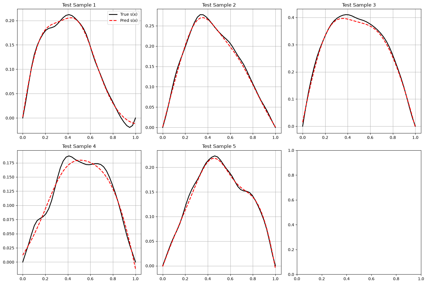
print("\n=== PREDICTION & EVALUATION ===")
s_pred, s_test, u_test, X_test = evaluate_model(model, train_data)

# Plot results
fig, axes = plt.subplots(2, 3, figsize=(15, 10))
for i in range(min(6, len(s_pred))):
    ax = axes[i//3, i%3]
    x_np = X_test[i].cpu().numpy()

    ax.plot(x_np, s_test[i].cpu().numpy(), 'k-', label='True s(x)', linewidth=2)
    ax.plot(x_np, s_pred[i].cpu().numpy(), 'r--', label='Pred s(x)', linewidth=2)

    ax.set_title(f'Test Sample {i+1}')
    ax.grid(True)
    if i == 0:
        ax.legend()

plt.tight_layout()
plt.savefig('deeponet_results.png', dpi=150)
plt.show()
=== PREDICTION & EVALUATION ===
Relative L2 error: 0.0345
Understanding basis functions#
def extract_basis_functions(model, X_test):
    """Extract and visualize learned basis functions"""
    device = next(model.parameters()).device
    model.eval()

    with torch.no_grad():
        # Use test locations
        x_points = X_test[0].unsqueeze(0).unsqueeze(-1).to(device)  # [1, n_points, 1]

        # Get trunk network output (basis functions)
        trunk_out = model.trunk(x_points)  # [1, n_points, p_dim]
        basis_functions = trunk_out.squeeze(0).cpu().numpy()  # [n_points, p_dim]

        print(f"Extracted {basis_functions.shape[1]} basis functions")
        print(f"Each basis function has {basis_functions.shape[0]} points")

        return basis_functions

print("\n=== BASIS FUNCTION ANALYSIS ===")
basis_functions = extract_basis_functions(model, X_test)

# Plot first 8 basis functions
fig, axes = plt.subplots(2, 4, figsize=(16, 8))
x_np = X_test[0].cpu().numpy()

for i in range(8):
    ax = axes[i//4, i%4]
    ax.plot(x_np, basis_functions[:, i], 'b-', linewidth=2)
    ax.set_title(f'Basis Function φ_{i+1}(y)')
    ax.grid(True)
    ax.set_xlabel('y')

plt.tight_layout()
plt.savefig('basis_functions.png', dpi=150)
plt.show()
=== BASIS FUNCTION ANALYSIS ===
Extracted 128 basis functions
Each basis function has 40 points
Summary:#
What We’ve Learned#
Conceptual Leap: From function approximation to operator learning
Functions: \(\mathbb{R}^d \rightarrow \mathbb{R}^m\) (point to point)
Operators: \(\mathcal{F}_1 \rightarrow \mathcal{F}_2\) (function to function)
Theoretical Foundation: Universal Approximation Theorem for Operators
Neural networks can approximate operators!
Branch-trunk architecture emerges naturally
Basis function decomposition: \(\mathcal{G}(u)(y) = \sum_k b_k(u) \cdot t_k(y)\)
Practical Implementation: DeepONet architecture
Branch network: Encodes input functions into coefficients
Trunk network: Generates basis functions at query points
Training: Learn from input-output function pairs
Real Applications: From derivatives to nonlinear PDEs
Derivative operator: Perfect pedagogical example
Darcy flow: Real-world nonlinear PDE
Generalization: Works on unseen function types
Key Advantages of DeepONet#
✅ Resolution independence: Train on one grid, evaluate on any grid
✅ Fast evaluation: Once trained, instant prediction
✅ Generalization: Works for new functions not seen during training
✅ Physical consistency: Learns the underlying operator, not just patterns
When to Use DeepONet#
Ideal scenarios:
Parametric PDEs: Need solutions for many different source terms/boundary conditions
Real-time applications: Require instant evaluation
Complex geometries: Traditional methods struggle
Multi-query problems: Same operator, many evaluations
Limitations:
Training data: Need many solved examples
Complex operators: Very nonlinear mappings may be challenging
High dimensions: Curse of dimensionality still applies
The Bigger Picture#
DeepONet represents a paradigm shift:
Traditional numerical methods: Solve each problem instance
Operator learning: Learn the solution pattern once, apply everywhere
This opens new possibilities for:
Inverse problems: Learn parameter-to-solution mappings
Control applications: Real-time system response
Multi-physics: Coupled operator learning
Scientific discovery: Understanding operator structure
Next: Combine with PINNs for physics-informed operator learning!
Further Reading and Extensions#
Key Papers#
Lu et al. (2019) - Original DeepONet paper
Goswami et al. (2023) - Physics-informed DeepONets
Chen & Chen (1995) - Universal approximation theorem for operators
Extensions to Explore#
Multi-output operators: Vector-valued mappings
Higher dimensions: 2D/3D PDEs
Physics-informed training: Incorporate governing equations
Fourier Neural Operators: Alternative operator learning architecture
Exercises#
Modify the derivative example to learn the second derivative operator
Extend to 2D by implementing the Laplacian operator \(\nabla^2 u\)
Add physics constraints by incorporating the differential equation into the loss
Compare with traditional methods on computational efficiency
The journey from function approximation to operator learning represents one of the most exciting frontiers in scientific machine learning!