ANY OpenSees from a Notebook

ANY OpenSees from a Notebook#

Running OpenSees & OpenSeesPy Input Scripts from a DesignSafe Jupyter Notebook

by Silvia Mazzoni, DesignSafe, 2025

This notebook shows how to run any OpenSees script — whether written in Tcl or Python (OpenSeesPy) — using Python’s built-in os library to execute commands just like in a terminal.

You can apply this technique in:

A Jupyter notebook, for an interactive and user-friendly experience
A standalone Python script, for automated or large-scale workflows

Why Use This Approach?#

It makes running OpenSees in the DesignSafe JupyterHub environment highly user-friendly
It lets you build seamless, Python-driven workflows that can include preprocessing, simulation, and postprocessing in one place
It works with any version of OpenSees already available in the Jupyter environment
You can also apply the same method to call OpenSees on an HPC system (e.g., Stampede3), making it easier to scale up or integrate into continuous workflows

Key Concepts:#

Use os.system() to call .tcl or .py input files from Python
Outputs go to the path defined in your script
%run (notebook magic) is more limited — it doesn’t accept arguments — so os.system() offers greater flexibility

Using local utilities library

cwd = os.getcwd()
print('current directory:',cwd)

current directory: /home/jupyter/MyData/_ToCommunityData/OpenSees/TrainingMaterial/training-OpenSees-on-DesignSafe/Jupyter_Notebooks

Define Base Path of Input Files.#

OpsScriptsPath = os.path.abspath('../Examples_OpenSees/BasicExamples')
print('OpsScriptsPath:',OpsScriptsPath)

OpsScriptsPath: /home/jupyter/MyData/_ToCommunityData/OpenSees/TrainingMaterial/training-OpenSees-on-DesignSafe/Examples_OpenSees/BasicExamples

Move to user’s home directory#

This way you can save files to your home path – you can’t write to CommunityData

os.chdir(os.path.expanduser('~')) # ~ the tilda is a shortcut to the uers's home path.
cwd = os.getcwd()
print('current directory:',cwd)

current directory: /home/jupyter

Create a temporary directory for our data and move to it#

We want the directory to be within MyData.

tmpDir = 'MyData/tmp_training'
os.makedirs(tmpDir, exist_ok=True)
os.chdir(tmpDir)
cwd = os.getcwd()
print('new current directory:',cwd)

new current directory: /home/jupyter/MyData/tmp_training

# !pip install OpenSeesPy (if needed)

Sequential#

TCL#

OpenSees.exe sequential#

inputFile = 'Ex1a.Canti2D.Push.tcl'

Ex1a.Canti2D.Push.tcl

# /home/jupyter/MyData/_ToCommunityData/OpenSees/TrainingMaterial/training-OpenSees-on-DesignSafe/Examples_OpenSees/BasicExamples/Ex1a.Canti2D.Push.tcl
# OpenSees Ex1a.Canti2D.Push.tcl

############################################################
#  EXAMPLE: 
#       Ex1a.Canti2D.Push.tcl
#          for OpenSees.exe (tcl)
#  --------------------------------------------------------#
#  by: Silvia Mazzoni, 2020
#       silviamazzoni@yahoo.com
############################################################
# This file was obtained by updating the Tcl script in the original examples manual
# You can find the original Examples:
# https://opensees.berkeley.edu/wiki/index.php/Examples_Manual
# Original Examples by By Silvia Mazzoni & Frank McKenna, 2006, in Tcl
############################################################
# --------------------------------------------------------------------------------------------------
# Example 1. cantilever 2D
# static pushover analysis with gravity.
# all units are in kip, inch, second
# elasticBeamColumn ELEMENT
#			Silvia Mazzoni & Frank McKenna, 2006
#
#    ^Y
#    |
#    2       __ 
#    |         | 
#    |         | 
#    |         | 
#  (1)      36'
#    |         | 
#    |         | 
#    |         | 
#  =1=    ----  -------->X
#
#

if {[llength $argv]>0} {
    puts "Command-Line Arguments (argv): $argv"
}

set LcolList "100 120 200 240 300 360 400 480"

# ----------------------------------------------
set dataDir DataTCL;                # set up name of data directory
file mkdir $dataDir; # create data directory

set count 0;
foreach Lcol $LcolList {
    
    # SET UP ----------------------------------------------------------------------------
    wipe;						# clear opensees model
    model basic -ndm 2 -ndf 3;	# 2 dimensions, 3 dof per node

    # define GEOMETRY -------------------------------------------------------------
    # nodal coordinates:
    node 1 0 0;				# node#, X Y
    node 2 0 $Lcol
    
    # Single point constraints -- Boundary Conditions
    fix 1 1 1 1; 			# node DX DY RZ
    
    # nodal masses:
    mass 2 5.18 0. 0.;		# node#, Mx My Mz, Mass=Weight/g.
    
    # Define ELEMENTS -------------------------------------------------------------
    # define geometric transformation: performs a linear geometric transformation of beam stiffness 
    #	and resisting force from the basic system to the global-coordinate system
    geomTransf Linear 1;  		# associate a tag to transformation
    
    # connectivity: (make A very large, 10e6 times its actual value)
    element elasticBeamColumn 1 1 2 3600000000 4227 1080000 1;	
    
    # Define RECORDERS -------------------------------------------------------------
    recorder Node -file ${dataDir}/DFree_Lcol${Lcol}.out -time -node 2 -dof 1 2 3 disp;			# displacements of free nodes
    recorder Node -file ${dataDir}/DBase_Lcol${Lcol}.out -time -node 1 -dof 1 2 3 disp;			# displacements of support nodes
    recorder Node -file ${dataDir}/RBase_Lcol${Lcol}.out -time -node 1 -dof 1 2 3 reaction;		# support reaction
    recorder Element -file ${dataDir}/FCol_Lcol${Lcol}.out -time -ele 1 globalForce;			# element forces -- column
    recorder Element -file ${dataDir}/DCol_Lcol${Lcol}.out -time -ele 1 deformation;			# element deformations -- column
    
    
    # define GRAVITY -------------------------------------------------------------
    timeSeries Linear 1;
    pattern Plain 1 1 {
       load 2 0. -2000. 0.;			# node#, FX FY MZ --  superstructure-weight
    }
    constraints Plain;     			# how it handles boundary conditions
    numberer Plain;					# renumber dof's to minimize band-width (optimization), if you want to
    system BandGeneral;				# how to store and solve the system of equations in the analysis
    test NormDispIncr 1.0e-8 6 ; 	# determine if convergence has been achieved at the end of an iteration step
    algorithm Newton;				# use Newton's solution algorithm: updates tangent stiffness at every iteration
    integrator LoadControl 0.1;		# determine the next time step for an analysis, # apply gravity in 10 steps
    analysis Static					# define type of analysis static or transient
    analyze 10;						# perform gravity analysis
    loadConst -time 0.0;			# hold gravity constant and restart time
    
    # define LATERAL load -------------------------------------------------------------
    timeSeries Linear 2;
    pattern Plain 2 2 {
        load 2 2000. 0.0 0.0;		# node#, FX FY MZ -- representative lateral load at top node
    }
    
    # pushover: diplacement controlled static analysis
    integrator DisplacementControl 2 1 0.1;		# switch to displacement control, for node 11, dof 1, 0.1 increment
    analyze 1000;								# apply 100 steps of pushover analysis to a displacement of 10
    
    puts "Analysis-${count} execution done"

    incr count 1;
}

puts "ALL DONE!!!"

os.system(f'OpenSees {OpsScriptsPath}/{inputFile}')

         OpenSees -- Open System For Earthquake Engineering Simulation
                 Pacific Earthquake Engineering Research Center
                        Version 3.7.1 64-Bit

      (c) Copyright 1999-2016 The Regents of the University of California
                              All Rights Reserved
  (Copyright and Disclaimer @ http://www.berkeley.edu/OpenSees/copyright.html)


Analysis-0 execution done
Analysis-1 execution done
Analysis-2 execution done
Analysis-3 execution done
Analysis-4 execution done
Analysis-5 execution done
Analysis-6 execution done
Analysis-7 execution done
ALL DONE!!!

Python#

OpenSeesPy sequential#

inputFile = 'Ex1a.Canti2D.Push.py'

Ex1a.Canti2D.Push.py

# /home/jupyter/MyData/_ToCommunityData/OpenSees/TrainingMaterial/training-OpenSees-on-DesignSafe/Examples_OpenSees/BasicExamples/Ex1a.Canti2D.Push.py
# python Ex1a.Canti2D.Push.py

############################################################
#  EXAMPLE: 
#       Ex1a.Canti2D.Push.py
#          for OpenSeesPy
#  --------------------------------------------------------#
#  by: Silvia Mazzoni, 2020
#       silviamazzoni@yahoo.com
############################################################
# This file was obtained from a conversion of the updated Tcl script
# You can find the original Examples:
# https://opensees.berkeley.edu/wiki/index.php/Examples_Manual
# Original Examples by By Silvia Mazzoni & Frank McKenna, 2006, in Tcl
# Converted to OpenSeesPy by SilviaMazzoni, 2020
############################################################
# --------------------------------------------------------------------------------------------------
# Example 1. cantilever 2D
# static pushover analysis with gravity.
# all units are in kip, inch, second
# elasticBeamColumn ELEMENT
#			Silvia Mazzoni & Frank McKenna, 2006
#
#    ^Y
#    |
#    2       __ 
#    |         | 
#    |         | 
#    |         | 
#  (1)      36'
#    |         | 
#    |         | 
#    |         | 
#  =1=    ----  -------->X
#
#

import openseespy.opensees as ops
import numpy as numpy
import matplotlib.pyplot as plt
import os
import sys

print(sys.argv)
if len(sys.argv)>1:
    print(f'Command-Line Arguments (argv): {sys.argv}')


LColList = [100,120,200,240,300,360,400,480]
#-----------------------------------------
dataDir=f'DataPY';                # set up name of data directory
os.makedirs(dataDir, exist_ok=True);    # create data directory

count = 0;
for Lcol in LColList:
    ops.wipe()

    # SET UP ----------------------------------------------------------------------------
    ops.wipe()     #  clear opensees model
    ops.model('basic','-ndm',2,'-ndf',3)     #  2 dimensions, 3 dof per node

    # define GEOMETRY -------------------------------------------------------------
    # nodal coordinates:
    ops.node(1,0,0)     #  node , X Y
    ops.node(2,0,Lcol)

    # Single point constraints -- Boundary Conditions
    ops.fix(1,1,1,1)     #  node DX DY RZ

    # nodal masses:
    ops.mass(2,5.18,0.,0.)     #  node , Mx My Mz, Mass=Weight/g.

    # Define ELEMENTS -------------------------------------------------------------
    # define geometric transformation: performs a linear geometric transformation of beam stiffness
    # and resisting force from the basic system to the global-coordinate system
    ops.geomTransf('Linear',1)     #  associate a tag to transformation

    # element elasticBeamColumn eleTag iNode jNode A E Iz transfTag
    ops.element('elasticBeamColumn',1,1,2,3600000000,4227,1080000,1)

    # Define RECORDERS -------------------------------------------------------------
    ops.recorder('Node','-file',f'{dataDir}/DFree_Lcol{Lcol}.out','-time','-node',2,'-dof',1,2,3,'disp')     #  displacements of free nodes
    ops.recorder('Node','-file',f'{dataDir}/DBase_Lcol{Lcol}.out','-time','-node',1,'-dof',1,2,3,'disp')     #  displacements of support nodes
    ops.recorder('Node','-file',f'{dataDir}/RBase_Lcol{Lcol}.out','-time','-node',1,'-dof',1,2,3,'reaction')     #  support reaction
    ops.recorder('Element','-file',f'{dataDir}/FCol_Lcol{Lcol}.out','-time','-ele',1,'globalForce')     #  element forces -- column
    ops.recorder('Element','-file',f'{dataDir}/DCol_Lcol{Lcol}.out','-time','-ele',1,'deformation')     #  element deformations -- column


    # define GRAVITY -------------------------------------------------------------
    ops.timeSeries('Linear',1)     # timeSeries Linear 1;
    ops.pattern('Plain',1,1) # 
    ops.load(2,0.,-2000.,0.)     #  node , FX FY MZ -- superstructure-weight
    ops.wipeAnalysis()     # adding this to clear Analysis module 
    ops.constraints('Plain')     #  how it handles boundary conditions
    ops.numberer('Plain')     #  renumber dofs to minimize band-width (optimization), if you want to
    ops.system('BandGeneral')     #  how to store and solve the system of equations in the analysis
    ops.test('NormDispIncr',1.0e-8,6)     #  determine if convergence has been achieved at the end of an iteration step
    ops.algorithm('Newton')     #  use Newtons solution algorithm: updates tangent stiffness at every iteration
    ops.integrator('LoadControl',0.1)     #  determine the next time step for an analysis,   apply gravity in 10 steps
    ops.analysis('Static')     #  define type of analysis static or transient
    ops.analyze(10)     #  perform gravity analysis
    ops.loadConst('-time',0.0)     #  hold gravity constant and restart time

    # define LATERAL load -------------------------------------------------------------
    ops.timeSeries('Linear',2)     # timeSeries Linear 2;
    ops.pattern('Plain',2,2) # 
    ops.load(2,2000.,0.0,0.0)     #  node , FX FY MZ -- representative lateral load at top node

    # pushover: diplacement controlled static analysis
    ops.integrator('DisplacementControl',2,1,0.1)     #  switch to displacement control, for node 11, dof 1, 0.1 increment
    ops.analyze(1000)     #  apply 100 steps of pushover analysis to a displacement of 10

    print(f'Analysis-{count} execution done')

    count +=1

print(f"ALL DONE!!!")

os.system(f'python {OpsScriptsPath}/{inputFile}')

['/home/jupyter/MyData/_ToCommunityData/OpenSees/TrainingMaterial/training-OpenSees-on-DesignSafe/Examples_OpenSees/BasicExamples/Ex1a.Canti2D.Push.py']
Analysis-0 execution done
Analysis-1 execution done
Analysis-2 execution done
Analysis-3 execution done
Analysis-4 execution done
Analysis-5 execution done
Analysis-6 execution done
Analysis-7 execution done
ALL DONE!!!

Process 0 Terminating

Parallel#

np=4 # number of processors

TCL#

OpenSeesMP parallel using mpiexec#

inputFile = 'Ex1a.Canti2D.Push.mp.tcl'

Ex1a.Canti2D.Push.mp.tcl

# /home/jupyter/MyData/_ToCommunityData/OpenSees/TrainingMaterial/training-OpenSees-on-DesignSafe/Examples_OpenSees/BasicExamples/Ex1a.Canti2D.Push.mp.tcl
# mpiexec -np 3 OpenSeesMP Ex1a.Canti2D.Push.mp.tcl

############################################################
#  EXAMPLE: 
#       Ex1a.Canti2D.Push.tcl
#          for OpenSees.exe (tcl)
#  --------------------------------------------------------#
#  by: Silvia Mazzoni, 2020
#       silviamazzoni@yahoo.com
############################################################
# This file was obtained by updating the Tcl script in the original examples manual
# You can find the original Examples:
# https://opensees.berkeley.edu/wiki/index.php/Examples_Manual
# Original Examples by By Silvia Mazzoni & Frank McKenna, 2006, in Tcl
############################################################
# --------------------------------------------------------------------------------------------------
# Example 1. cantilever 2D
# static pushover analysis with gravity.
# all units are in kip, inch, second
# elasticBeamColumn ELEMENT
#			Silvia Mazzoni & Frank McKenna, 2006
#
#    ^Y
#    |
#    2       __ 
#    |         | 
#    |         | 
#    |         | 
#  (1)      36'
#    |         | 
#    |         | 
#    |         | 
#  =1=    ----  -------->X
#
#



set pid [getPID]
set np [getNP]
puts "pid $pid of np=$np  started"


if {[llength $argv]>0} {
    puts "pid $pid of np=$np  Command-Line Arguments (argv): $argv"
}

set LcolList "100 120 200 240 300 360 400 480"

# ----------------------------------------------
set dataDir DataTCLmp;                # set up name of data directory
file mkdir $dataDir; # create data directory

set count 0;
foreach Lcol $LcolList {
    # check if count is a multiple of pid : "is it its turn?"
    if {[expr $count % $np] == $pid} {
       
        # SET UP ----------------------------------------------------------------------------
        wipe;						# clear opensees model
        model basic -ndm 2 -ndf 3;	# 2 dimensions, 3 dof per node
        
        # define GEOMETRY -------------------------------------------------------------
        # nodal coordinates:
        node 1 0 0;				# node#, X Y
        node 2 0 $Lcol
        
        # Single point constraints -- Boundary Conditions
        fix 1 1 1 1; 			# node DX DY RZ
        
        # nodal masses:
        mass 2 5.18 0. 0.;		# node#, Mx My Mz, Mass=Weight/g.
        
        # Define ELEMENTS -------------------------------------------------------------
        # define geometric transformation: performs a linear geometric transformation of beam stiffness 
        #	and resisting force from the basic system to the global-coordinate system
        geomTransf Linear 1;  		# associate a tag to transformation
        
        # connectivity: (make A very large, 10e6 times its actual value)
        # element elasticBeamColumn $eleTag $iNode $jNode $A $E $Iz $transfTag
        element elasticBeamColumn 1 1 2 3600000000 4227 1080000 1;	
        
        # Define RECORDERS -------------------------------------------------------------
        recorder Node -file ${dataDir}/DFree_Lcol${Lcol}.out -time -node 2 -dof 1 2 3 disp;			# displacements of free nodes
        recorder Node -file ${dataDir}/DBase_Lcol${Lcol}.out -time -node 1 -dof 1 2 3 disp;			# displacements of support nodes
        recorder Node -file ${dataDir}/RBase_Lcol${Lcol}.out -time -node 1 -dof 1 2 3 reaction;		# support reaction
        recorder Element -file ${dataDir}/FCol_Lcol${Lcol}.out -time -ele 1 globalForce;			# element forces -- column
        recorder Element -file ${dataDir}/DCol_Lcol${Lcol}.out -time -ele 1 deformation;			# element deformations -- column
        
        
        # define GRAVITY -------------------------------------------------------------
        timeSeries Linear 1;
        pattern Plain 1 1 {
           load 2 0. -2000. 0.;			# node#, FX FY MZ --  superstructure-weight
        }
        constraints Plain;     			# how it handles boundary conditions
        numberer Plain;					# renumber dof's to minimize band-width (optimization), if you want to
        system BandGeneral;				# how to store and solve the system of equations in the analysis
        test NormDispIncr 1.0e-8 6 ; 	# determine if convergence has been achieved at the end of an iteration step
        algorithm Newton;				# use Newton's solution algorithm: updates tangent stiffness at every iteration
        integrator LoadControl 0.1;		# determine the next time step for an analysis, # apply gravity in 10 steps
        analysis Static					# define type of analysis static or transient
        analyze 10;						# perform gravity analysis
        loadConst -time 0.0;			# hold gravity constant and restart time
        
        # define LATERAL load -------------------------------------------------------------
        timeSeries Linear 2;
        pattern Plain 2 2 {
           load 2 2000. 0.0 0.0;		# node#, FX FY MZ -- representative lateral load at top node
        }
        
        # pushover: diplacement controlled static analysis
        integrator DisplacementControl 2 1 0.1;		# switch to displacement control, for node 11, dof 1, 0.1 increment
        analyze 1000;								# apply 100 steps of pushover analysis to a displacement of 10
        
        puts "pid $pid of $np Analysis-${count} execution done"
        
        
    }
    incr count 1;
}

puts "pid $pid ALL DONE!!!"

os.system(f'mpiexec -np {np} OpenSeesMP {OpsScriptsPath}/{inputFile}')

         OpenSees -- Open System For Earthquake Engineering Simulation
                 Pacific Earthquake Engineering Research Center
                        Version 3.7.1 64-Bit

      (c) Copyright 1999-2016 The Regents of the University of California
                              All Rights Reserved
  (Copyright and Disclaimer @ http://www.berkeley.edu/OpenSees/copyright.html)


pid 2 of np=4  started
pid 1 of np=4  started
pid 0 of np=4  started
pid 3 of np=4  started
pid 0 of 4 Analysis-0 execution done
pid 2 of 4 Analysis-2 execution done
pid 1 of 4 Analysis-1 execution done
pid 3 of 4 Analysis-3 execution done
pid 0 of 4 Analysis-4 execution done
pid 0 ALL DONE!!!
Process Terminating 0
pid 2 of 4 Analysis-6 execution done
pid 2 ALL DONE!!!
Process Terminating 2
pid 1 of 4 Analysis-5 execution done
pid 1 ALL DONE!!!
Process Terminating 1
pid 3 of 4 Analysis-7 execution done
pid 3 ALL DONE!!!
Process Terminating 3

f'mpiexec -np {np} OpenSeesMP {OpsScriptsPath}/{inputFile}'

'mpiexec -np 4 OpenSeesMP /home/jupyter/MyData/_ToCommunityData/OpenSees/TrainingMaterial/training-OpenSees-on-DesignSafe/Examples_OpenSees/BasicExamples/Ex1a.Canti2D.Push.mp.tcl'

Python#

OpenSeesPy parallel using mpiexec#

inputFile = 'Ex1a.Canti2D.Push.mpi.py'

Ex1a.Canti2D.Push.mpi.py

# /home/jupyter/MyData/_ToCommunityData/OpenSees/TrainingMaterial/training-OpenSees-on-DesignSafe/Examples_OpenSees/BasicExamples/Ex1a.Canti2D.Push.mpi.py
# mpiexec -np 3 python Ex1a.Canti2D.Push.mpi.py

import openseespy.opensees as ops
import numpy as numpy
import matplotlib.pyplot as plt
import sys
import os

ops.start()
pid = ops.getPID()
np = ops.getNP()
print(f'pid {pid} of {np} started')

if len(sys.argv)>1:
    print(f'mpi -- python pid {pid} of {np} Command-Line Arguments (argv): {sys.argv}')

LColList = [100,120,200,240,300,360,400,480]
#-----------------------------------------
dataDir=f'DataPYmpi';                # set up name of data directory
os.makedirs(dataDir, exist_ok=True); # create data directory

count = 0;
for Lcol in LColList:
    # check if count is a multiple of pid : "is it its turn?"
    if count % np == pid:
        ops.wipe()
        
        # SET UP ----------------------------------------------------------------------------
        ops.wipe()     #  clear opensees model
        ops.model('basic','-ndm',2,'-ndf',3)     #  2 dimensions, 3 dof per node
        
        
        # define GEOMETRY -------------------------------------------------------------
        # nodal coordinates:
        ops.node(1,0,0)     #  node , X Y
        ops.node(2,0,Lcol)
        
        # Single point constraints -- Boundary Conditions
        ops.fix(1,1,1,1)     #  node DX DY RZ
        
        # nodal masses:
        ops.mass(2,5.18,0.,0.)     #  node , Mx My Mz, Mass=Weight/g.
        
        # Define ELEMENTS -------------------------------------------------------------
        # define geometric transformation: performs a linear geometric transformation of beam stiffness
        # and resisting force from the basic system to the global-coordinate system
        ops.geomTransf('Linear',1)     #  associate a tag to transformation
        
        # element elasticBeamColumn eleTag iNode jNode A E Iz transfTag
        ops.element('elasticBeamColumn',1,1,2,3600000000,4227,1080000,1)
        
        # Define RECORDERS -------------------------------------------------------------
        ops.recorder('Node','-file',f'{dataDir}/DFree_Lcol{Lcol}.out','-time','-node',2,'-dof',1,2,3,'disp')     #  displacements of free nodes
        ops.recorder('Node','-file',f'{dataDir}/DBase_Lcol{Lcol}.out','-time','-node',1,'-dof',1,2,3,'disp')     #  displacements of support nodes
        ops.recorder('Node','-file',f'{dataDir}/RBase_Lcol{Lcol}.out','-time','-node',1,'-dof',1,2,3,'reaction')     #  support reaction
        ops.recorder('Element','-file',f'{dataDir}/FCol_Lcol{Lcol}.out','-time','-ele',1,'globalForce')     #  element forces -- column
        ops.recorder('Element','-file',f'{dataDir}/DCol_Lcol{Lcol}.out','-time','-ele',1,'deformation')     #  element deformations -- column
        
        # define GRAVITY -------------------------------------------------------------
        ops.timeSeries('Linear',1)     # timeSeries Linear 1;
        ops.pattern('Plain',1,1) # 
        ops.load(2,0.,-2000.,0.)     #  node , FX FY MZ -- superstructure-weight
        ops.wipeAnalysis()     # adding this to clear Analysis module 
        ops.constraints('Plain')     #  how it handles boundary conditions
        ops.numberer('Plain')     #  renumber dofs to minimize band-width (optimization), if you want to
        ops.system('BandGeneral')     #  how to store and solve the system of equations in the analysis
        ops.test('NormDispIncr',1.0e-8,6)     #  determine if convergence has been achieved at the end of an iteration step
        ops.algorithm('Newton')     #  use Newtons solution algorithm: updates tangent stiffness at every iteration
        ops.integrator('LoadControl',0.1)     #  determine the next time step for an analysis,   apply gravity in 10 steps
        ops.analysis('Static')     #  define type of analysis static or transient
        ops.analyze(10)     #  perform gravity analysis
        ops.loadConst('-time',0.0)     #  hold gravity constant and restart time
        
        # define LATERAL load -------------------------------------------------------------
        ops.timeSeries('Linear',2)     # timeSeries Linear 2;
        ops.pattern('Plain',2,2) # 
        ops.load(2,2000.,0.0,0.0)     #  node , FX FY MZ -- representative lateral load at top node
        
        # pushover: diplacement controlled static analysis
        ops.integrator('DisplacementControl',2,1,0.1)     #  switch to displacement control, for node 11, dof 1, 0.1 increment
        ops.analyze(1000)     #  apply 100 steps of pushover analysis to a displacement of 10
        
        print(f'pid {pid} of np={np} Analysis-{count} execution done')

    count +=1

print(f"pid {pid} of np={np} ALL DONE!!!")

os.system(f'mpiexec -np {np} python {OpsScriptsPath}/{inputFile}')
print('If you only see "pid=0" and "np=1", then the MPI implementation failed!')

pid 0 of 1 started
pid 0 of 1 started
pid 0 of np=1 Analysis-0 execution done
pid 0 of np=1 Analysis-0 execution done
pid 0 of np=1 Analysis-1 execution done
pid 0 of 1 started
pid 0 of np=1 Analysis-1 execution done
pid 0 of 1 started
pid 0 of np=1 Analysis-2 execution done
pid 0 of np=1 Analysis-0 execution done
pid 0 of np=1 Analysis-0 execution done
pid 0 of np=1 Analysis-3 execution done
pid 0 of np=1 Analysis-2 execution done
pid 0 of np=1 Analysis-1 execution done
pid 0 of np=1 Analysis-4 execution done
pid 0 of np=1 Analysis-1 execution done
pid 0 of np=1 Analysis-3 execution done
pid 0 of np=1 Analysis-2 execution done
pid 0 of np=1 Analysis-5 execution done
pid 0 of np=1 Analysis-4 execution done
pid 0 of np=1 Analysis-3 execution done
pid 0 of np=1 Analysis-2 execution done
pid 0 of np=1 Analysis-6 execution done
pid 0 of np=1 Analysis-4 execution done
pid 0 of np=1 Analysis-5 execution done
pid 0 of np=1 Analysis-3 execution done
pid 0 of np=1 Analysis-7 execution done
pid 0 of np=1 ALL DONE!!!
pid 0 of np=1 Analysis-6 execution done
pid 0 of np=1 Analysis-5 execution done
pid 0 of np=1 Analysis-4 execution done
pid 0 of np=1 Analysis-6 execution done
pid 0 of np=1 Analysis-7 execution done
pid 0 of np=1 ALL DONE!!!
pid 0 of np=1 Analysis-5 execution done
pid 0 of np=1 Analysis-7 execution done
pid 0 of np=1 ALL DONE!!!
pid 0 of np=1 Analysis-6 execution done
pid 0 of np=1 Analysis-7 execution done
pid 0 of np=1 ALL DONE!!!
If you only see "pid=0" and "np=1", then the MPI implementation failed!

Process 0 Terminating
Process 0 Terminating
Process 0 Terminating
Process 0 Terminating

OpenSeesPy parallel using mpi4py#

inputFile = 'Ex1a.Canti2D.Push.mpi4py.py'

Ex1a.Canti2D.Push.mpi4py.py

# /home/jupyter/MyData/_ToCommunityData/OpenSees/TrainingMaterial/training-OpenSees-on-DesignSafe/Examples_OpenSees/BasicExamples/Ex1a.Canti2D.Push.mpi4py.py
# mpiexec -np 3 python Ex1a.Canti2D.Push.mpi4py.py

import openseespy.opensees as ops
import numpy as numpy
import matplotlib.pyplot as plt
import sys
import os

from mpi4py import MPI
comm = MPI.COMM_WORLD
pid = comm.Get_rank()
np=comm.Get_size()
print(f'mpi4py -- python pid {pid} of {np} started')

if len(sys.argv)>1:
    print(f'mpi4py -- python pid {pid} of {np} Command-Line Arguments (argv): {sys.argv}')


LColList = [100,120,200,240,300,360,400,480]
#-----------------------------------------
dataDir=f'DataPYmpi4py';                # set up name of data directory
os.makedirs(dataDir, exist_ok=True);    # create data directory

count = 0;
for Lcol in LColList:
    # check if count is a multiple of pid : "is it its turn?"
    if count % np == pid:
        ops.wipe()
        
        # SET UP ----------------------------------------------------------------------------
        ops.wipe()     #  clear opensees model
        ops.model('basic','-ndm',2,'-ndf',3)     #  2 dimensions, 3 dof per node
        
        
        # define GEOMETRY -------------------------------------------------------------
        # nodal coordinates:
        ops.node(1,0,0)     #  node , X Y
        ops.node(2,0,Lcol)
        
        # Single point constraints -- Boundary Conditions
        ops.fix(1,1,1,1)     #  node DX DY RZ
        
        # nodal masses:
        ops.mass(2,5.18,0.,0.)     #  node , Mx My Mz, Mass=Weight/g.
        
        # Define ELEMENTS -------------------------------------------------------------
        # define geometric transformation: performs a linear geometric transformation of beam stiffness
        # and resisting force from the basic system to the global-coordinate system
        ops.geomTransf('Linear',1)     #  associate a tag to transformation
        
        # connectivity: (make A very large, 10e6 times its actual value)
        ops.element('elasticBeamColumn',1,1,2,3600000000,4227,1080000,1)
        
        # Define RECORDERS -------------------------------------------------------------
        ops.recorder('Node','-file',f'{dataDir}/DFree_Lcol{Lcol}.out','-time','-node',2,'-dof',1,2,3,'disp')     #  displacements of free nodes
        ops.recorder('Node','-file',f'{dataDir}/DBase_Lcol{Lcol}.out','-time','-node',1,'-dof',1,2,3,'disp')     #  displacements of support nodes
        ops.recorder('Node','-file',f'{dataDir}/RBase_Lcol{Lcol}.out','-time','-node',1,'-dof',1,2,3,'reaction')     #  support reaction
        ops.recorder('Element','-file',f'{dataDir}/FCol_Lcol{Lcol}.out','-time','-ele',1,'globalForce')     #  element forces -- column
        ops.recorder('Element','-file',f'{dataDir}/DCol_Lcol{Lcol}.out','-time','-ele',1,'deformation')     #  element deformations -- column

        
        # define GRAVITY -------------------------------------------------------------
        ops.timeSeries('Linear',1)     # timeSeries Linear 1;
        ops.pattern('Plain',1,1) # 
        ops.load(2,0.,-2000.,0.)     #  node , FX FY MZ -- superstructure-weight
        ops.wipeAnalysis()     # adding this to clear Analysis module 
        ops.constraints('Plain')     #  how it handles boundary conditions
        ops.numberer('Plain')     #  renumber dofs to minimize band-width (optimization), if you want to
        ops.system('BandGeneral')     #  how to store and solve the system of equations in the analysis
        ops.test('NormDispIncr',1.0e-8,6)     #  determine if convergence has been achieved at the end of an iteration step
        ops.algorithm('Newton')     #  use Newtons solution algorithm: updates tangent stiffness at every iteration
        ops.integrator('LoadControl',0.1)     #  determine the next time step for an analysis,   apply gravity in 10 steps
        ops.analysis('Static')     #  define type of analysis static or transient
        ops.analyze(10)     #  perform gravity analysis
        ops.loadConst('-time',0.0)     #  hold gravity constant and restart time
        
        # define LATERAL load -------------------------------------------------------------
        ops.timeSeries('Linear',2)     # timeSeries Linear 2;
        ops.pattern('Plain',2,2) # 
        ops.load(2,2000.,0.0,0.0)     #  node , FX FY MZ -- representative lateral load at top node
        
        # pushover: diplacement controlled static analysis
        ops.integrator('DisplacementControl',2,1,0.1)     #  switch to displacement control, for node 11, dof 1, 0.1 increment
        ops.analyze(1000)     #  apply 100 steps of pushover analysis to a displacement of 10
        
        print(f'pid {pid} of np={np} Analysis-{count} execution done')

    count +=1

print(f"pid {pid} of np={np} ALL DONE!!!")

os.system(f'mpiexec -np {np} python {OpsScriptsPath}/{inputFile}')

mpi4py -- python pid 0 of 4 started
mpi4py -- python pid 1 of 4 started
mpi4py -- python pid 3 of 4 started
mpi4py -- python pid 2 of 4 started
pid 2 of np=4 Analysis-2 execution done
pid 1 of np=4 Analysis-1 execution done
pid 0 of np=4 Analysis-0 execution done
pid 3 of np=4 Analysis-3 execution done
pid 1 of np=4 Analysis-5 execution done
pid 1 of np=4 ALL DONE!!!
pid 0 of np=4 Analysis-4 execution done
pid 0 of np=4 ALL DONE!!!
pid 2 of np=4 Analysis-6 execution done
pid 2 of np=4 ALL DONE!!!
pid 3 of np=4 Analysis-7 execution done
pid 3 of np=4 ALL DONE!!!

Process 0 Terminating
Process 0 Terminating
Process 0 Terminating
Process 0 Terminating

Run OpenSeesPy script within this notebook#

running the script in this manner maintains all variable definitions and OpenSees-Model Objects (unless wipe was used)

inputFile = 'Ex1a.Canti2D.Push.py'

Ex1a.Canti2D.Push.py

# /home/jupyter/MyData/_ToCommunityData/OpenSees/TrainingMaterial/training-OpenSees-on-DesignSafe/Examples_OpenSees/BasicExamples/Ex1a.Canti2D.Push.py
# python Ex1a.Canti2D.Push.py

############################################################
#  EXAMPLE: 
#       Ex1a.Canti2D.Push.py
#          for OpenSeesPy
#  --------------------------------------------------------#
#  by: Silvia Mazzoni, 2020
#       silviamazzoni@yahoo.com
############################################################
# This file was obtained from a conversion of the updated Tcl script
# You can find the original Examples:
# https://opensees.berkeley.edu/wiki/index.php/Examples_Manual
# Original Examples by By Silvia Mazzoni & Frank McKenna, 2006, in Tcl
# Converted to OpenSeesPy by SilviaMazzoni, 2020
############################################################
# --------------------------------------------------------------------------------------------------
# Example 1. cantilever 2D
# static pushover analysis with gravity.
# all units are in kip, inch, second
# elasticBeamColumn ELEMENT
#			Silvia Mazzoni & Frank McKenna, 2006
#
#    ^Y
#    |
#    2       __ 
#    |         | 
#    |         | 
#    |         | 
#  (1)      36'
#    |         | 
#    |         | 
#    |         | 
#  =1=    ----  -------->X
#
#

import openseespy.opensees as ops
import numpy as numpy
import matplotlib.pyplot as plt
import os
import sys

print(sys.argv)
if len(sys.argv)>1:
    print(f'Command-Line Arguments (argv): {sys.argv}')


LColList = [100,120,200,240,300,360,400,480]
#-----------------------------------------
dataDir=f'DataPY';                # set up name of data directory
os.makedirs(dataDir, exist_ok=True);    # create data directory

count = 0;
for Lcol in LColList:
    ops.wipe()

    # SET UP ----------------------------------------------------------------------------
    ops.wipe()     #  clear opensees model
    ops.model('basic','-ndm',2,'-ndf',3)     #  2 dimensions, 3 dof per node

    # define GEOMETRY -------------------------------------------------------------
    # nodal coordinates:
    ops.node(1,0,0)     #  node , X Y
    ops.node(2,0,Lcol)

    # Single point constraints -- Boundary Conditions
    ops.fix(1,1,1,1)     #  node DX DY RZ

    # nodal masses:
    ops.mass(2,5.18,0.,0.)     #  node , Mx My Mz, Mass=Weight/g.

    # Define ELEMENTS -------------------------------------------------------------
    # define geometric transformation: performs a linear geometric transformation of beam stiffness
    # and resisting force from the basic system to the global-coordinate system
    ops.geomTransf('Linear',1)     #  associate a tag to transformation

    # element elasticBeamColumn eleTag iNode jNode A E Iz transfTag
    ops.element('elasticBeamColumn',1,1,2,3600000000,4227,1080000,1)

    # Define RECORDERS -------------------------------------------------------------
    ops.recorder('Node','-file',f'{dataDir}/DFree_Lcol{Lcol}.out','-time','-node',2,'-dof',1,2,3,'disp')     #  displacements of free nodes
    ops.recorder('Node','-file',f'{dataDir}/DBase_Lcol{Lcol}.out','-time','-node',1,'-dof',1,2,3,'disp')     #  displacements of support nodes
    ops.recorder('Node','-file',f'{dataDir}/RBase_Lcol{Lcol}.out','-time','-node',1,'-dof',1,2,3,'reaction')     #  support reaction
    ops.recorder('Element','-file',f'{dataDir}/FCol_Lcol{Lcol}.out','-time','-ele',1,'globalForce')     #  element forces -- column
    ops.recorder('Element','-file',f'{dataDir}/DCol_Lcol{Lcol}.out','-time','-ele',1,'deformation')     #  element deformations -- column


    # define GRAVITY -------------------------------------------------------------
    ops.timeSeries('Linear',1)     # timeSeries Linear 1;
    ops.pattern('Plain',1,1) # 
    ops.load(2,0.,-2000.,0.)     #  node , FX FY MZ -- superstructure-weight
    ops.wipeAnalysis()     # adding this to clear Analysis module 
    ops.constraints('Plain')     #  how it handles boundary conditions
    ops.numberer('Plain')     #  renumber dofs to minimize band-width (optimization), if you want to
    ops.system('BandGeneral')     #  how to store and solve the system of equations in the analysis
    ops.test('NormDispIncr',1.0e-8,6)     #  determine if convergence has been achieved at the end of an iteration step
    ops.algorithm('Newton')     #  use Newtons solution algorithm: updates tangent stiffness at every iteration
    ops.integrator('LoadControl',0.1)     #  determine the next time step for an analysis,   apply gravity in 10 steps
    ops.analysis('Static')     #  define type of analysis static or transient
    ops.analyze(10)     #  perform gravity analysis
    ops.loadConst('-time',0.0)     #  hold gravity constant and restart time

    # define LATERAL load -------------------------------------------------------------
    ops.timeSeries('Linear',2)     # timeSeries Linear 2;
    ops.pattern('Plain',2,2) # 
    ops.load(2,2000.,0.0,0.0)     #  node , FX FY MZ -- representative lateral load at top node

    # pushover: diplacement controlled static analysis
    ops.integrator('DisplacementControl',2,1,0.1)     #  switch to displacement control, for node 11, dof 1, 0.1 increment
    ops.analyze(1000)     #  apply 100 steps of pushover analysis to a displacement of 10

    print(f'Analysis-{count} execution done')

    count +=1

print(f"ALL DONE!!!")

exec(open(f'{OpsScriptsPath}/{inputFile}').read())

['/opt/conda/lib/python3.12/site-packages/ipykernel_launcher.py', '-f', '/home/jupyter/.local/share/jupyter/runtime/kernel-be779e07-1d1b-4a88-93d5-24c6a488f9d5.json']
Command-Line Arguments (argv): ['/opt/conda/lib/python3.12/site-packages/ipykernel_launcher.py', '-f', '/home/jupyter/.local/share/jupyter/runtime/kernel-be779e07-1d1b-4a88-93d5-24c6a488f9d5.json']
Analysis-0 execution done
Analysis-1 execution done
Analysis-2 execution done
Analysis-3 execution done
Analysis-4 execution done
Analysis-5 execution done
Analysis-6 execution done
Analysis-7 execution done
ALL DONE!!!

Variables & OpenSees model have been preserved:

# OpenSees Model have been preserved (unless wipe has been used)
print('OpenSees Model')
ops.printModel()

OpenSees Model

Current Domain Information
	Current Time: 6.19189
	Committed Time: 6.19189
NODE DATA: NumNodes: 2

numComponents: 2

 Node: 1
	Coordinates  : 0 0 
	Disps: 0 0 0 
	 unbalanced Load: 0 0 0 
	 reaction: -12383.8 2000 5.94422e+06 
	ID : -1 -1 -1 


 Node: 2
	Coordinates  : 0 480 
	Disps: 100 -6.30865e-08 -0.3125 
	 unbalanced Load: 12383.8 -2000 0 
	 reaction: -1.81899e-12 2.27374e-13 -4.65661e-10 
	Mass : 
5.18 0 0 
0 0 0 
0 0 0 

	 Rayleigh Factor: alphaM: 0
	 Rayleigh Forces: 0 0 0 
	ID : 0 1 2 

ELEMENT DATA: NumEle: 1

numComponents: 1

ElasticBeam2d: 1
	Connected Nodes: 1 2 
	CoordTransf: 1
	mass density:  0, cMass: 0
	release code:  0
	End 1 Forces (P V M): 2000 12383.8 5.94422e+06
	End 2 Forces (P V M): -2000 -12383.8 -4.65661e-10

SP_Constraints: numConstraints: 3

numComponents: 3
SP_Constraint: 0	 Node: 1 DOF: 1 ref value: 0 current value: 0 initial value: 0
SP_Constraint: 1	 Node: 1 DOF: 2 ref value: 0 current value: 0 initial value: 0
SP_Constraint: 2	 Node: 1 DOF: 3 ref value: 0 current value: 0 initial value: 0

Pressure_Constraints: numConstraints: 0

numComponents: 0

MP_Constraints: numConstraints: 0

numComponents: 0

LOAD PATTERNS: numPatterns: 2


numComponents: 2
Load Pattern: 1
  Scale Factor: 1
Linear Series: constant factor: 1
  Nodal Loads: 

numComponents: 1
Nodal Load: 2 load : 0 -2000 0 

  Elemental Loads: 

numComponents: 0

  Single Point Constraints: 

numComponents: 0
Load Pattern: 2
  Scale Factor: 1
Linear Series: constant factor: 1
  Nodal Loads: 

numComponents: 1
Nodal Load: 2 load : 2000 0 0 

  Elemental Loads: 

numComponents: 0

  Single Point Constraints: 

numComponents: 0

PARAMETERS: numParameters: 0


numComponents: 0

Plot analysis results#

for any of the above analyses

#pick any case
dataDir = 'DataTCL'
Lcol = 400

# check paths:
print('relative path:',os.path.expanduser(dataDir))
print('absolute path:',os.path.abspath(dataDir))

print('current directory:',os.getcwd())

relative path: DataTCL
absolute path: /home/jupyter/MyData/tmp_training/DataTCL
current directory: /home/jupyter/MyData/tmp_training

plt.close('all')
fname3 = f'{dataDir}/DFree_Lcol{Lcol}.out'
dataDFree = numpy.loadtxt(fname3)
plt.subplot(211)
plt.title(f'Ex1a.Canti2D {dataDir}')
plt.grid(True)
plt.plot(dataDFree[:,1])
plt.xlabel('Step Number')
plt.ylabel('Free-Node Displacement')
plt.subplot(212)
plt.grid(True)
plt.plot(dataDFree[:,1],dataDFree[:,0])
plt.xlabel('Free-Node Disp.')
plt.ylabel('Pseudo-Time (~Force)')
plt.savefig(f'{dataDir}/Response.jpg')
plt.show()
print(f'plot saved to {dataDir}/Response_Lcol{Lcol}.jpg')
print('End of Run: Ex1a.Canti2D.Push.py.ipynb')

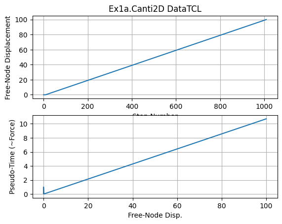
../_images/6ec66cb1653d5c2ec2821d8579303b3c8d1e47b9773064808a171a2ada9336af.png

plot saved to DataTCL/Response_Lcol400.jpg
End of Run: Ex1a.Canti2D.Push.py.ipynb

ANY OpenSees from a Notebook

Contents

ANY OpenSees from a Notebook#

Why Use This Approach?#

Key Concepts:#

Define Base Path of Input Files.#

Move to user’s home directory#

Create a temporary directory for our data and move to it#

Sequential#

TCL#

OpenSees.exe sequential#

Python#

OpenSeesPy sequential#

Parallel#

TCL#

OpenSeesMP parallel using mpiexec#

Python#

OpenSeesPy parallel using mpiexec#

OpenSeesPy parallel using mpi4py#

Run OpenSeesPy script within this notebook#

Plot analysis results#