4 PostProcess Ops-Express#
Take advantage of the interactive nature of the Jupyter environment to visualize output data quantitatively.
by Silvia Mazzoni, DesignSafe, 2025
In this training session we will visualize the job-output data before copying it over.
This is an important step because it helps you determine whether the job was run as intended. If not, you can resubmit a job without moving the data, yet.
Configure python#
import matplotlib.pyplot as plt
import numpy
Using local utilities library
# add the tilda at the beginning of the path to make it absolute
JobOutputFolder = '~/MyData/tapis-jobs-archive/2025-07-28Z/OpenSees_opensees-express-latest_2025-07-28T20:09:24-b17040ea-8d34-4916-9664-7caaee938467-007/BasicExamples'
print('JobOutputFolder',JobOutputFolder)
# list some files:
print('Folder Content:')
display(os.system(f'ls {JobOutputFolder}'))
JobOutputFolder ~/MyData/tapis-jobs-archive/2025-07-28Z/OpenSees_opensees-express-latest_2025-07-28T20:09:24-b17040ea-8d34-4916-9664-7caaee938467-007/BasicExamples
Folder Content:
DataTCL
Ex1a.Canti2D.Push.mp.tcl
Ex1a.Canti2D.Push.mpi.py
Ex1a.Canti2D.Push.mpi4py.py
Ex1a.Canti2D.Push.py
Ex1a.Canti2D.Push.tcl
Ex1a_many.Canti2D.Push.mp.tcl
0
4. Copy base path for output data from posted path:#
basePath = os.path.expanduser(JobOutputFolder)
print('basePath',basePath)
basePath /home/jupyter/MyData/tapis-jobs-archive/2025-07-28Z/OpenSees_opensees-express-latest_2025-07-28T20:09:24-b17040ea-8d34-4916-9664-7caaee938467-007/BasicExamples
os.path.isdir(basePath)
True
os.listdir(basePath)
['DataTCL',
 'Ex1a_many.Canti2D.Push.mp.tcl',
 'Ex1a.Canti2D.Push.mpi4py.py',
 'Ex1a.Canti2D.Push.mp.tcl',
 'Ex1a.Canti2D.Push.mpi.py',
 'Ex1a.Canti2D.Push.py',
 'Ex1a.Canti2D.Push.tcl']
Visualize the Input File#
Ex1a.Canti2D.Push.tcl
# /home/jupyter/MyData/tapis-jobs-archive/2025-07-28Z/OpenSees_opensees-express-latest_2025-07-28T20:09:24-b17040ea-8d34-4916-9664-7caaee938467-007/BasicExamples/Ex1a.Canti2D.Push.tcl
# OpenSees Ex1a.tcl.Canti2D.Push.tcl

############################################################
#  EXAMPLE:
#       Ex1a.Canti2D.Push.tcl
#          for OpenSees.exe (tcl)
#  --------------------------------------------------------#
#  by: Silvia Mazzoni, 2020
#       silviamazzoni@yahoo.com
############################################################
# This file was obtained by updating the Tcl script in the original examples manual
# You can find the original Examples:
# https://opensees.berkeley.edu/wiki/index.php/Examples_Manual
# Original Examples by By Silvia Mazzoni & Frank McKenna, 2006, in Tcl
############################################################
# --------------------------------------------------------------------------------------------------
# Example 1. cantilever 2D
# static pushover analysis with gravity.
# all units are in kip, inch, second
# elasticBeamColumn ELEMENT
#			Silvia Mazzoni & Frank McKenna, 2006
#
#    ^Y
#    |
#    2       __
#    |         |
#    |         |
#    |         |
#  (1)      36'
#    |         |
#    |         |
#    |         |
#  =1=    ----  -------->X
#
#


set LcolList "100 120 200 240 300 360 400 480"

# ----------------------------------------------
set dataDir DataTCL;                # set up name of data directory
file mkdir $dataDir; # create data directory

set count 0;
foreach Lcol $LcolList {

    # SET UP ----------------------------------------------------------------------------
    wipe;						# clear opensees model
    model basic -ndm 2 -ndf 3;	# 2 dimensions, 3 dof per node

    # define GEOMETRY -------------------------------------------------------------
    # nodal coordinates:
    node 1 0 0;				# node#, X Y
    node 2 0 $Lcol

    # Single point constraints -- Boundary Conditions
    fix 1 1 1 1; 			# node DX DY RZ

    # nodal masses:
    mass 2 5.18 0. 0.;		# node#, Mx My Mz, Mass=Weight/g.

    # Define ELEMENTS -------------------------------------------------------------
    # define geometric transformation: performs a linear geometric transformation of beam stiffness
    #	and resisting force from the basic system to the global-coordinate system
    geomTransf Linear 1;  		# associate a tag to transformation

    # connectivity: (make A very large, 10e6 times its actual value)
    element elasticBeamColumn 1 1 2 3600000000 4227 1080000 1;

    # Define RECORDERS -------------------------------------------------------------
    recorder Node -file ${dataDir}/DFree_Lcol${Lcol}.out -time -node 2 -dof 1 2 3 disp;			# displacements of free nodes
    recorder Node -file ${dataDir}/DBase_Lcol${Lcol}.out -time -node 1 -dof 1 2 3 disp;			# displacements of support nodes
    recorder Node -file ${dataDir}/RBase_Lcol${Lcol}.out -time -node 1 -dof 1 2 3 reaction;		# support reaction
    recorder Element -file ${dataDir}/FCol_Lcol${Lcol}.out -time -ele 1 globalForce;			# element forces -- column
    recorder Element -file ${dataDir}/DCol_Lcol${Lcol}.out -time -ele 1 deformation;			# element deformations -- column


    # define GRAVITY -------------------------------------------------------------
    timeSeries Linear 1;
    pattern Plain 1 1 {
       load 2 0. -2000. 0.;			# node#, FX FY MZ --  superstructure-weight
    }
    constraints Plain;     			# how it handles boundary conditions
    numberer Plain;					# renumber dof's to minimize band-width (optimization), if you want to
    system BandGeneral;				# how to store and solve the system of equations in the analysis
    test NormDispIncr 1.0e-8 6 ; 	# determine if convergence has been achieved at the end of an iteration step
    algorithm Newton;				# use Newton's solution algorithm: updates tangent stiffness at every iteration
    integrator LoadControl 0.1;		# determine the next time step for an analysis, # apply gravity in 10 steps
    analysis Static					# define type of analysis static or transient
    analyze 10;						# perform gravity analysis
    loadConst -time 0.0;			# hold gravity constant and restart time

    # define LATERAL load -------------------------------------------------------------
    timeSeries Linear 2;
    pattern Plain 2 2 {
        load 2 2000. 0.0 0.0;		# node#, FX FY MZ -- representative lateral load at top node
    }

    # pushover: diplacement controlled static analysis
    integrator DisplacementControl 2 1 0.1;		# switch to displacement control, for node 11, dof 1, 0.1 increment
    analyze 1000;								# apply 100 steps of pushover analysis to a displacement of 10

    puts "Analysis-${count} execution done"

    incr count 1;
}

puts "ALL DONE!!!"
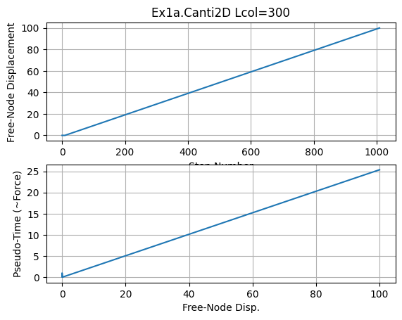
5. Plot some analysis results#
for any of the above analyses
#pick any case
dataDir = f'{basePath}/DataTCL'
Lcol = 300
print('dataDir',dataDir)
# list some files:
os.system(f'ls {dataDir}/*Lcol{Lcol}.out')
dataDir /home/jupyter/MyData/tapis-jobs-archive/2025-07-28Z/OpenSees_opensees-express-latest_2025-07-28T20:09:24-b17040ea-8d34-4916-9664-7caaee938467-007/BasicExamples/DataTCL
/home/jupyter/MyData/tapis-jobs-archive/2025-07-28Z/OpenSees_opensees-express-latest_2025-07-28T20:09:24-b17040ea-8d34-4916-9664-7caaee938467-007/BasicExamples/DataTCL/DBase_Lcol300.out
/home/jupyter/MyData/tapis-jobs-archive/2025-07-28Z/OpenSees_opensees-express-latest_2025-07-28T20:09:24-b17040ea-8d34-4916-9664-7caaee938467-007/BasicExamples/DataTCL/DCol_Lcol300.out
/home/jupyter/MyData/tapis-jobs-archive/2025-07-28Z/OpenSees_opensees-express-latest_2025-07-28T20:09:24-b17040ea-8d34-4916-9664-7caaee938467-007/BasicExamples/DataTCL/DFree_Lcol300.out
/home/jupyter/MyData/tapis-jobs-archive/2025-07-28Z/OpenSees_opensees-express-latest_2025-07-28T20:09:24-b17040ea-8d34-4916-9664-7caaee938467-007/BasicExamples/DataTCL/FCol_Lcol300.out
/home/jupyter/MyData/tapis-jobs-archive/2025-07-28Z/OpenSees_opensees-express-latest_2025-07-28T20:09:24-b17040ea-8d34-4916-9664-7caaee938467-007/BasicExamples/DataTCL/RBase_Lcol300.out
0
plt.close('all')
fname3o = f'DFree_Lcol{Lcol}.out'
fname3 = f'{dataDir}/{fname3o}'
print(fname3)
dataDFree = numpy.loadtxt(fname3)
plt.subplot(211)
plt.title(f'Ex1a.Canti2D Lcol={Lcol}')
plt.grid(True)
plt.plot(dataDFree[:,1])
plt.xlabel('Step Number')
plt.ylabel('Free-Node Displacement')
plt.subplot(212)
plt.grid(True)
plt.plot(dataDFree[:,1],dataDFree[:,0])
plt.xlabel('Free-Node Disp.')
plt.ylabel('Pseudo-Time (~Force)')
plt.savefig(f'{dataDir}/Response.jpg')
plt.show()
print(f'plot saved to {dataDir}/Response_Lcol{Lcol}.jpg')
print('End of Run: Ex1a.Canti2D.Push.py.ipynb')
/home/jupyter/MyData/tapis-jobs-archive/2025-07-28Z/OpenSees_opensees-express-latest_2025-07-28T20:09:24-b17040ea-8d34-4916-9664-7caaee938467-007/BasicExamples/DataTCL/DFree_Lcol300.out
plot saved to /home/jupyter/MyData/tapis-jobs-archive/2025-07-28Z/OpenSees_opensees-express-latest_2025-07-28T20:09:24-b17040ea-8d34-4916-9664-7caaee938467-007/BasicExamples/DataTCL/Response_Lcol300.jpg
End of Run: Ex1a.Canti2D.Push.py.ipynb
print('Done!')
Done!